Comparing Biases for Minimal Network Construction with Back-Propagation

Hanson S J, Pratt L Y. Comparing Biases for Minimal Network Construction with Back-Propagation. Advances in Neural Information Processing Systems 1, 1988.

Neural NetworkBack-PropagationWeight DecayMinimal NetworkNIPS 1988BellcoreRutgers

反向传播最小网络构建中的偏置比较

Abstract

Rumelhart (1987) has proposed a method for choosing minimal or "simple" representations during learning in Back-propagation networks. This approach can be used to (a) dynamically select the number of hidden units, (b) construct a representation that is appropriate for the problem and (c) thus improve the generalization ability of Back-propagation networks. The method Rumelhart suggests involves adding penalty terms to the usual error function. In this paper we introduce Rumelhart's minimal networks idea and compare two possible biases on the weight search space. These biases are compared in both simple counting problems and a speech recognition problem. In general, the constrained search does seem to minimize the number of hidden units required with an expected increase in local minima.

Rumelhart（1987）提出了一种方法，用于在反向传播网络的学习过程中选择最小或“简单”的表征。该方法可用于：(a) 动态选择隐藏单元数量；(b) 构建适合当前问题的表征；以及 (c) 由此提高反向传播网络的泛化能力。 Rumelhart 建议的方法是在通常的误差函数中加入惩罚项。在本文中，我们介绍 Rumelhart 的最小网络思想，并比较权重搜索空间上的两种可能偏置。我们在简单计数问题和语音识别问题上比较这些偏置。总体而言，约束搜索似乎确实减少了所需隐藏单元的数量，但预期会增加局部极小值。

Introduction

Many supervised connectionist models use gradient descent in error to solve various kinds of tasks (Rumelhart, Hinton & Williams, 1986). However, such gradient descent methods tend to be "opportunistic" and can solve problems in an arbitrary way dependent on starting point in weight space and peculiarities of the training set. For example, in Figure Figure 1 we show a "mesh" problem which consists of a random distribution of exemplars from two categories. The spatial geometry of the categories impose a meshed or overlapping subset of the exemplars in the two dimensional feature space. As the meshed part of the categories increase the problem becomes more complex and must involve the combination of more linear cuts in feature space and consequently more nonlinear cuts for category separation. In the top left corner of Figure Figure 1(a), we show a mesh geometry requiring only three cuts for category separation. In the bottom center Figure Figure 1(b) is the projection of the three cut solution of the mesh in output space. In the top right of this Figure Figure 1(c) is a typical solution provided by back-propagation starting with 16 hidden units. This Figure shows the two dimensional feature space in which 9 of the linear cuts are projected (the other 7 are outside the $[0, 1]$ unit plane).

许多监督式联结主义模型使用误差梯度下降来解决各种任务（Rumelhart、Hinton 和 Williams，1986）。然而，这类梯度下降方法往往具有“机会主义”特征，会以任意方式解决问题，而其方式取决于权重空间中的起点和训练集的特殊性。例如，在图1 中，我们展示了一个“网格”问题，它由两个类别中随机分布的样本组成。这些类别的空间几何结构使二维特征空间中的一部分样本形成网格状或重叠分布。随着类别网格部分增大，问题变得更加复杂，必须在特征空间中组合更多线性切分，并相应使用更多非线性切分来分离类别。在图1(a) 左上角，我们展示了一个只需三次切分即可实现类别分离的网格几何结构。图1(b) 位于下方中央，是网格三切分解在输出空间中的投影。图1(c) 位于右上方，是从 16 个隐藏单元开始进行反向传播所得的一个典型解。该图展示了二维特征空间，其中投影了 9 条线性切分线（另有 7 条位于 $[0, 1]$ 单位平面之外）。

Mesh problem, output space, and a typical back-propagation solution — 图1：Mesh problem (a), output space (b) and typical back-propagation solution (c)

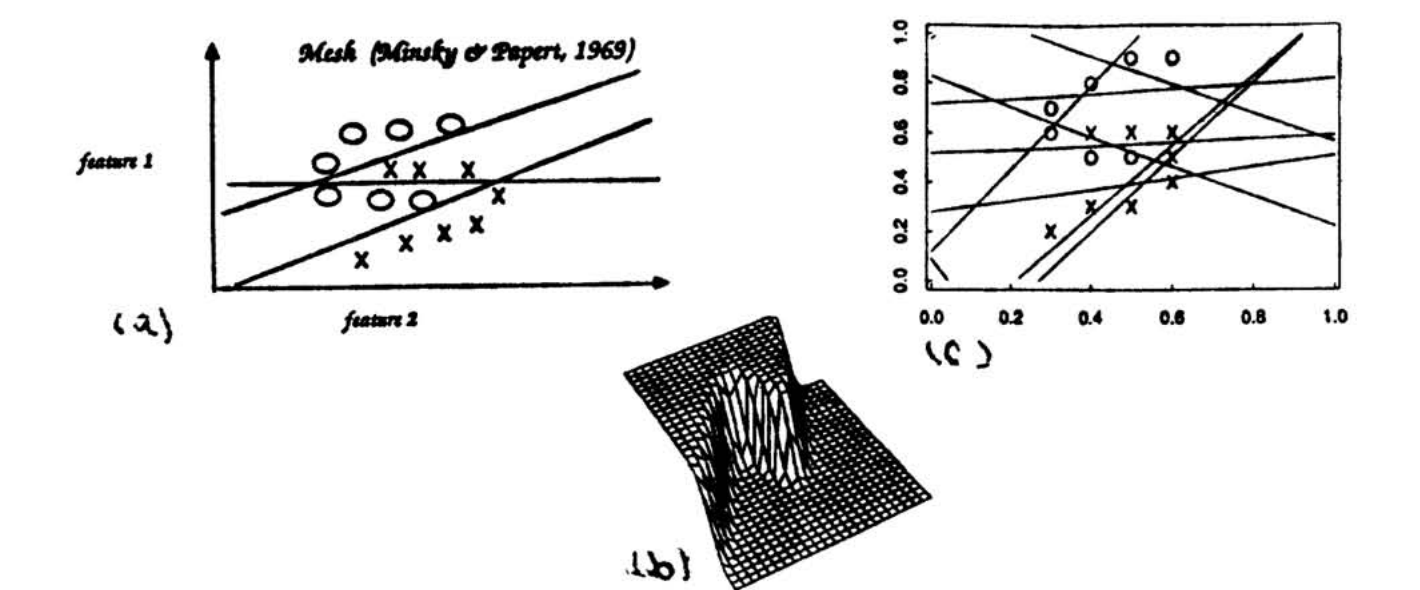
Examining the weights in the next layer of the network indicates that in fact, 7 of these 9 line segments are used in order to construct the output surface shown in Figure Figure 1(b). Consequently, the underlying feature relations determining the output surface and category separation are arbitrary, more complex than necessary and may result in anomalous generalizations.

检查网络下一层的权重可以发现，为构建图1(b) 所示的输出曲面，实际上使用了这 9 条线段中的 7 条。因此，决定输出曲面和类别分离的底层特征关系是任意的，比必要情况更复杂，并且可能产生异常泛化。

Rumelhart (1987) has proposed a way to increase the generalization capabilities of learning networks which use gradient descent methods and to automatically control the resources learning networks use -- for example, in terms of "hidden" units. His hypothesis concerns the nature of the representation in the network: "... the simplest most robust network which accounts for a data set will, on average, lead to the best generalization to the population from which the training set has been drawn".

Rumelhart（1987）提出了一种方法，可以提高采用梯度下降方法的学习网络的泛化能力，并自动控制学习网络使用的资源，例如“隐藏”单元的数量。他的假设涉及网络中表征的性质：“……能够解释一个数据集的最简单、最稳健网络，平均而言，将对抽取该训练集的总体产生最佳泛化。”

The basic approach involves adding penalty terms to the usual error function in order to constrain the search and cause weights to differentially decay. This is similar to many proposals in statistical regression where a "simplicity" measure is minimized along with the error term and is sometimes referred to as "biased" regression (Rawlings, 1988). Basically, the statistical concept of biased regression derives from parameter estimation approaches that attempt to achieve a best linear unbiased estimator ("BLUE"). By definition an unbiased estimator is one with the lowest possible variance and theoretically, unless there is significant collinearity or nonlinearity amongst the variables, a least squares estimator (LSE) can be also shown to be a BLUE. If on the other hand, input variables are correlated or nonlinear with the output variables (as is the case in back-propagation) then there is no guarantee that the LSE will also be unbiased. Consequently, introducing a bias may actually reduce the variance of the estimator of that below the theoretically unbiased estimator.

基本方法是在通常的误差函数中加入惩罚项，以约束搜索并使权重产生差异化衰减。这与统计回归中的许多方案相似：在最小化误差项的同时最小化一种“简单性”度量，这有时称为“有偏”回归（Rawlings，1988）。从根本上说，有偏回归这一统计概念源自试图得到最佳线性无偏估计量（BLUE）的参数估计方法。根据定义，无偏估计量具有尽可能低的方差；理论上，除非变量之间存在显著共线性或非线性，否则最小二乘估计量（LSE）也可以被证明是 BLUE。另一方面，如果输入变量与输出变量相关或呈非线性关系（反向传播正是如此），则无法保证 LSE 仍然无偏。因此，引入偏置实际上可能把估计量的方差降低到理论无偏估计量之下。

Footnote 1. For example, Ridge regression is a special case of biased regression which attempts to make a singular correlation matrix non-singular by adding a small arbitrary constant to the diagonal of the matrix. This increase in the diagonal may lower the impact of the off-diagonal elements and thus reduce the effects of collinearity.

注 1。 例如，岭回归是有偏回归的一种特殊情形，它通过在矩阵对角线上加入一个任意的小常数，试图使奇异相关矩阵变为非奇异矩阵。对角线上的这种增量可能降低非对角元素的影响，从而减弱共线性的作用。

Since back-propagation is a special case of multivariate nonlinear regression methods we must immediately give up on achieving a BLUE. Worse yet, the input variables are also very likely to be collinear in that input data are typically expected to be used for feature extraction. Consequently, the neural network framework leads naturally to the exploration of biased regression techniques; unfortunately, it is not obvious what sorts of biases ought to be introduced and whether they may be problem dependent. Furthermore, the choice of particular biases probably determines the particular representation that is chosen and its nature in terms of size, structure and "simplicity". This representation bias may in turn induce generalization behavior which is greater in accuracy with larger coverage over the domain. Nonetheless, since there is no particular motivation for minimizing a least squares estimator it is important to begin exploring possible biases that would lead to lower variance and more robust estimators.

由于反向传播是多元非线性回归方法的一种特殊情形，我们必须立即放弃获得 BLUE 的目标。更糟的是，输入变量也很可能具有共线性，因为输入数据通常预期被用于特征提取。因此，神经网络框架自然会引向对有偏回归技术的探索；遗憾的是，应当引入何种偏置以及它们是否依赖具体问题并不明确。此外，具体偏置的选择可能决定最终选择的具体表征，以及该表征在规模、结构和“简单性”方面的性质。这种表征偏置进而可能诱导出准确率更高、领域覆盖范围更大的泛化行为。尽管如此，由于没有必须最小化最小二乘估计量的特定理由，因此有必要开始探索能够带来更低方差和更稳健估计量的偏置。

In this paper we explore two general type of bias which introduce explicit constraints on the hidden units. First we discuss the standard back-propagation method, various past methods of biasing which have been called "weight decay", the properties of our biases, and finally some simple benchmark tests using parity and a speech recognition task.

在本文中，我们探索两类对隐藏单元施加显式约束的一般偏置。我们首先讨论标准反向传播方法、过去被称为“权重衰减”的多种偏置方法以及我们所用偏置的性质，最后给出采用奇偶校验和语音识别任务的简单基准测试。

Back-Propagation

The Back-propagation method is a supervised learning technique using a gradient descent in an error variable. The error is established by comparing an output value to a desired or expected value. These errors can be accumulated over the sample:

反向传播方法是一种在误差变量上使用梯度下降的监督学习技术。误差通过比较输出值与期望值来确定。这些误差可以在样本上累积：

\begin{matrix} (1) & E = \sum_{s} \sum_{i} {(y_{i s} - {\hat{y}}_{i s})}^{2} . \end{matrix}

Assuming the output function is differentiable then a gradient of the error can be found, and we require that this derivative be decreasing.

假设输出函数可微，则可以求得误差的梯度，并且我们要求该导数递减。

\begin{matrix} (2) & - \frac{\partial E}{\partial w_{i j}} = 0 . \end{matrix}

Over multiple layers we pass back a weighted sum of each derivative from units above.

跨越多层时，我们向后传递来自上层单元的各个导数的加权和。

Weight Decay

Past work using biases have generally been based on ad hoc arguments that weights should differentially decay allowing large weights to persist and small weights to tend towards zero sooner. Apparently, this would tend to concentrate more of the input into a smaller number of weights. Generally, the intuitive notion is to somehow reduce the complexity of the network as defined by the number of connections and number of hidden units. A simple but inefficient way of doing this is to include a weight decay term in the usual delta updating rule causing all weights to decay on each learning step (where $w = w_{i j}$ throughout):

过去采用偏置的工作通常建立在一种临时性论点上：权重应当差异化衰减，使大权重得以保留，而小权重更快趋近于零。显然，这会倾向于把更多输入集中到较少的权重上。一般而言，其直观想法是以某种方式降低由连接数和隐藏单元数定义的网络复杂度。一种简单但低效的方法，是在通常的 delta 更新规则中加入权重衰减项，使所有权重在每个学习步骤中都发生衰减（全文令 $w = w_{i j}$ ）：

\begin{matrix} (3) & w_{n + 1} = α {(- \frac{\partial E}{\partial w})}_{n} + β w_{n} . \end{matrix}

Solving this difference equation shows that for $β < 1.0$ weights are decaying exponentially over steps towards zero.

求解该差分方程可知，当 $β < 1.0$ 时，权重会随步骤以指数方式衰减至零。

\begin{matrix} (4) & w_{n} = α \sum_{i = 1}^{n} β^{n - i} {(- \frac{\partial E}{\partial w})}_{i} + β^{n} w_{0} . \end{matrix}

This approach introduces the decay term in the derivative itself causing error terms to also decrease over learning steps which may not be desirable.

这种方法把衰减项引入导数本身，使误差项也随学习步骤减小，而这可能并非理想行为。

Footnote 2. Most of the work discussed here has not been previously published but nonetheless has entered into general use in many connectionist models and was recently summarized on the Connectionist Bulletin Board by John Kruschke.

注 2。 这里讨论的大部分工作此前并未发表，但已经普遍用于许多联结主义模型，John Kruschke 最近在 Connectionist Bulletin Board 上对此作了总结。

Bias

The sort of weight decay just discussed can also be derived from general consideration of "costs" on weights. For example it is possible to consider $E$ with a bias term which in the simple decay case is quadratic with weight value (i.e. $w^{2}$ ).

刚才讨论的权重衰减也可以从权重“代价”的一般考虑中推导出来。例如，可以为 $E$ 加入一个偏置项；在简单衰减情形下，该项是权重值的二次函数（即 $w^{2}$ ）。

We now combine this bias with $E$ producing an objective function that includes both the error term and this bias function:

现在，我们把该偏置与 $E$ 结合，得到一个同时包含误差项和偏置函数的目标函数：

\begin{matrix} (5) & O = E + B . \end{matrix}

Where, we now want to minimize

此时，我们要最小化

\begin{matrix} (6) & \frac{\partial O}{\partial w_{i j}} = \frac{\partial E}{\partial w_{i j}} + \frac{\partial B}{\partial w_{i j}} . \end{matrix}

In the quadratic case the updating rule becomes,

在二次函数情形下，更新规则变为：

\begin{matrix} (7) & w_{n + 1} = α (- \frac{\partial E}{\partial w_{i j}} - 2 w_{n}) + w_{n} . \end{matrix}

Solving this difference equation derives the updating rule from equation 4.

求解该差分方程即可得到式 (4) 中的更新规则。

\begin{matrix} (8) & w_{n} = α \sum_{i = 1}^{n} (1 - 2 α)^{n - i} {(- \frac{\partial E}{\partial w_{i j}})}_{i} + (1 - 2 α)^{n} w_{0} . \end{matrix}

In this case, however without introduction of other parameters, $α$ is both the learning rate and related to the decay term and must be strictly $< \frac{1}{2}$ for weight decay.

然而在这种情况下，如果不引入其他参数， $α$ 既是学习率又与衰减项相关，并且要实现权重衰减，它必须严格小于 $\frac{1}{2}$ 。

Uniform weight decay has a disadvantage in that large weights are decaying at the same rate as small weights. It is possible to design biases that influence weights only when they are relatively small or even in a particular range of values. For example, Rumelhart has entertained a number of biases, one form in particular that we will also explore is based on a rectangular hyperbolic function.

均匀权重衰减的一个缺点是，大权重与小权重以相同速率衰减。我们可以设计仅在权重相对较小、甚至仅在某个特定取值范围内才影响权重的偏置。例如，Rumelhart 考察过多种偏置，其中我们也将探索的一种形式基于矩形双曲函数。

\begin{matrix} (9) & B = \frac{w^{2}}{1 + w^{2}} . \end{matrix}

It is informative to examine the derivative associated with this function in order to understand its effect on the weight updates.

为了理解该函数对权重更新的影响，考察与它相关的导数很有启发性。

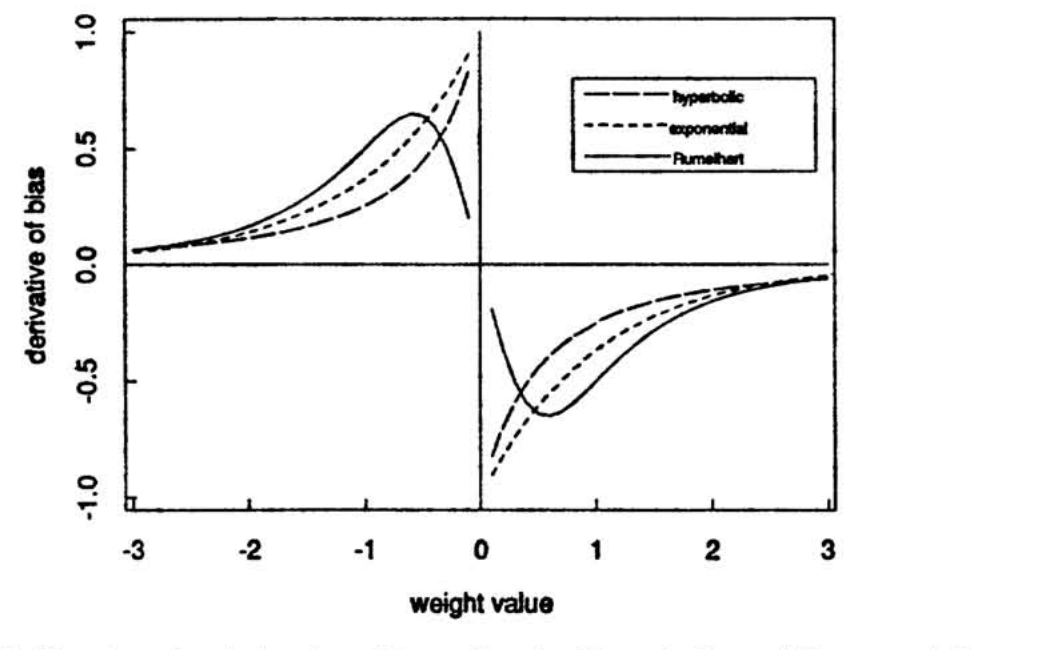
\begin{matrix} (10) & - \frac{\partial B}{\partial w_{i j}} = - \frac{2 w}{(1 + w^{2})^{2}} . \end{matrix}

This derivative is plotted in Figure Figure 2 (indicated as Rumelhart) and is non-monotonic showing a strong differential effect on small weights (+ or -) pushing them towards zero, while near zero and large weight values are not significantly affected.

该导数绘制于图2 中（标为 Rumelhart）；它是非单调的，对较小的正、负权重产生强烈差异化作用并将其推向零，而接近零的权重和较大的权重值不会受到显著影响。

Bias per Unit

It is possible to consider bias on each hidden unit weight group. This has the potentially desirable effect of isolating weight changes to hidden unit weight groups and could effectively eliminate hidden units. Consequently, the hidden units are directly determining the bias. In order to do this, first define

可以在每个隐藏单元权重组上考虑偏置。这样做可能带来一种理想效果：把权重变化限制在隐藏单元权重组内，并且能够有效消除隐藏单元。因此，隐藏单元会直接决定偏置。为此，首先定义

\begin{matrix} (11) & w_{i} = \sum_{j} | w_{i j} | . \end{matrix}

Where $i$ is the $i$ th hidden unit.

其中， $i$ 表示第 $i$ 个隐藏单元。

Hyperbolic Bias

Now consider a function similar to Rumelhart's but this time with $w_{i}$ , the $i$ th hidden group as the variable.

现在考虑一个与 Rumelhart 所用函数相似的函数，但这次以第 $i$ 个隐藏组 $w_{i}$ 为变量。

\begin{matrix} (12) & B = \frac{w_{i}}{1 + λ w_{i}} . \end{matrix}

The new gradient includes the term from the bias which is,

新的梯度包含来自偏置的如下项：

\begin{matrix} (13) & - \frac{\partial B}{\partial w_{i j}} = - \frac{λ sgn (w_{i j})}{(1 + w_{i})^{2}} . \end{matrix}

Exponential Bias

A similar kind of bias would be to consider the negative exponential:

另一种类似偏置可以采用负指数形式：

\begin{matrix} (14) & B = 1 - e^{- λ w_{i}} . \end{matrix}

This bias is similar to the hyperbolic bias term as above but involves the exponential which potentially produce more uniform and gradual rate changes towards zero.

该偏置与上面的双曲偏置项相似，但它采用指数函数，因而可能产生更均匀、更渐进的趋零速率变化。

\begin{matrix} (15) & - \frac{\partial B}{\partial w_{i j}} = - \frac{sgn (w_{i j})}{e^{λ w_{i}}} . \end{matrix}

The behavior of these two biases (hyperbolic, exponential) are shown as function of weight magnitudes in Figure Figure 2. Notice that the exponential bias term is more similar in slope change to Rumelhart's (even though his is non-monotonic) than the hyperbolic as weight magnitude to a hidden unit increases.

这两种偏置（双曲偏置和指数偏置）随权重幅值变化的行为如图2 所示。请注意，随着连接到某一隐藏单元的权重幅值增大，指数偏置项的斜率变化比双曲偏置更接近 Rumelhart 的偏置项（尽管后者是非单调的）。

Derivative behavior of Rumelhart, hyperbolic, and exponential bias functions — 图2：Bias function behavior of Rumelhart's, Hyperbolic and Exponential

Obviously there are many more kinds of bias that one can consider. These two were chosen in order to provide a systematic test of varying biases and exploring their differential effectiveness in minimizing network complexity.

显然，还可以考虑更多种类的偏置。选择这两种偏置，是为了系统测试不同偏置，并探索它们在降低网络复杂度方面的差异化效果。

Some Comparisons: Parity

These biased Back-propagation methods were applied to several counting problems and to a speech (digit) recognition problem. In the following graphs for example, we show the results of 100 runs of XOR and 4-bit parity at $η = .1$ (learning rate) and $α = .8$ (moving average) starting with 10 hidden units. The parameter $λ$ was optimized for the bias runs.

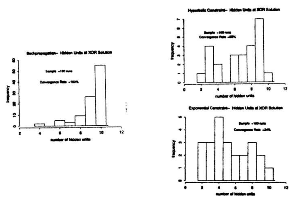
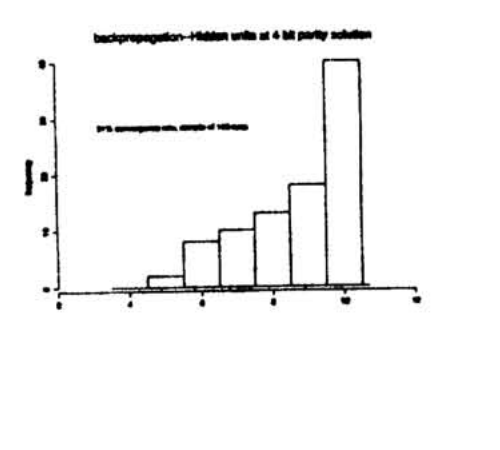
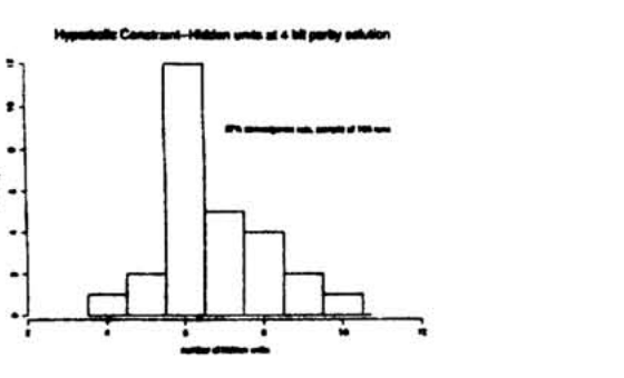
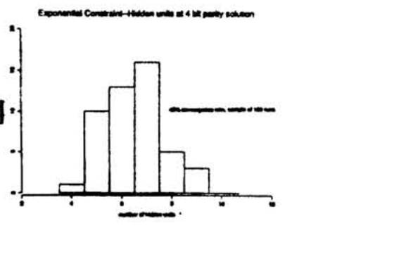
这些带偏置的反向传播方法被应用于若干计数问题和一个语音（数字）识别问题。例如，在下面的图中，我们展示了从 10 个隐藏单元开始、以 $η = .1$ （学习率）和 $α = .8$ （移动平均）进行 100 次 XOR 与四位奇偶校验运行的结果。参数 $λ$ 针对偏置运行进行了优化。

Exclusive OR runs for standard, hyperbolic, and exponential biasing — 图3：Exclusive OR runs for standard, hyperbolic and exponential biasing

Shown are runs for the standard case without biases, the hyperbolic bias and the exponential bias. Once a solution was reached all hidden units were tested individually by removing each of them one at a time from the network and then testing on the training set. Any hidden unit which was unnecessary was removed for data analysis. Only the number of these "functional units" are reported in the histograms. Notice the number of hidden units decrease with bias runs. An analysis of variance (statistical test) verified this improvement for both the hyperbolic and exponential over the standard. Also note that the exponential is significantly better than the hyperbolic. This is also confirmed for the 4-bit parity case as shown in Figure Figure 4.

图中给出了无偏置的标准情形、双曲偏置和指数偏置的运行结果。得到解之后，我们逐一从网络中移除每个隐藏单元，并在训练集上测试，从而分别检验所有隐藏单元。数据分析时会移除任何不必要的隐藏单元。直方图只报告这些“功能单元”的数量。可以看到，采用偏置时隐藏单元数量减少。方差分析（一种统计检验）证实，相比标准方法，双曲偏置和指数偏置都带来了这种改进。还可以看到，指数偏置显著优于双曲偏置。图4 所示的四位奇偶校验情形也证实了这一点。

Standard back-propagation runs for four-bit parity — 图4：Four-bit parity runs for standard, hyperbolic and exponential biasing

Hyperbolic bias runs for four-bit parity — 图4：Four-bit parity runs for standard, hyperbolic and exponential biasing

Speech Recognition

Samples of 10 spoken digits (0-9) each were collected (same speaker throughout -- D. J. Burr kindly supplied data). Samples were then preprocessed using FFTs retaining the first 12 Cepstral coefficients. To avoid ceiling effects only two tokens each of the 10 digits were used for training ("0", "0", "1", "1", ..., "9", "9") each network. Eight such 2 token samples were used for replications. Another set of 50 spoken digits (5 samples of each of the 10 digits) were collected for transfer. All runs were matched across methods for number of learning sweeps ( $< 300$ ), $η = .05$ , $α = .2$ , and $λ = .01$ which were optimized for the exponential bias. Shown in the following table is the results of the 8 replications for the standard and the exponential bias.

我们收集了数字 0 至 9 各自的语音样本（始终由同一说话人发音，D. J. Burr 慷慨提供了数据）。随后使用快速傅里叶变换预处理样本，并保留前 12 个倒谱系数。为避免天花板效应，每个网络在训练时只使用 10 个数字各两个语音样本（“0”“0”“1”“1”……“9”“9”）。我们使用八组这样的双样本数据进行重复实验。另行收集了 50 个语音数字（10 个数字各 5 个样本）用于迁移测试。所有方法的运行都匹配学习轮数（ $< 300$ ）、 $η = .05$ 、 $α = .2$ 和 $λ = .01$ ；这些参数针对指数偏置进行了优化。下面的表1 给出了标准方法和指数偏置方法八次重复实验的结果。

表1：Eight replications with transfer for standard and exponential bias.

	Back-propagation		Constrained (exp.)
Sample	Transfer	# Hidden Units	Transfer	# Hidden Units
r1	50%	18	64%	10
r2	60%	17	76%	13
r3	62%	18	64%	14
r4	66%	14	74%	14
r5	62%	16	56%	11
r6	66%	19	68%	14
r7	58%	18	54%	11
r8	58%	18	64%	9
Mean ± s.e.	59% ± 1.9	17 ± .56	65% ± 2.8	12 ± .71

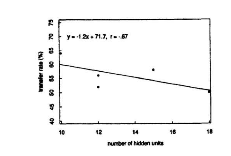
In this case there appears to both an improvement in the average number of hidden units (functional ones) and transfer. A typical correlation of the improved transfer and reduced hidden unit usage for a single replication is plotted in the next graph.

在这种情况下，隐藏单元（功能单元）的平均数量和迁移性能似乎都得到了改善。下一幅图绘制了一次重复实验中迁移性能提高与隐藏单元使用量减少之间的典型相关关系。

Transfer rate as a function of the number of hidden units — 图5：Transfer as a function of hidden unit usage for a single replication

We note that introduction of biases decrease the probability of convergence relative to the standard case (as many as 75% of the parity runs did not converge within criteria number of sweeps.) Since the search problem is made more difficult by introducing biases it now becomes even more important to explore methods for improving convergence similar for example, to simulated annealing (Kirkpatrick, Gelatt & Vecchi, 1983).

我们注意到，与标准情形相比，引入偏置会降低收敛概率（多达 75% 的奇偶校验运行未能在判定轮数内收敛）。由于引入偏置会使搜索问题更加困难，因此探索提高收敛性的方法变得更加重要，例如采用类似模拟退火的方法（Kirkpatrick、Gelatt 和 Vecchi，1983）。

Conclusions

Minimal networks were defined and two types of bias were compared in a simple counting problem and a speech recognition problem. In the counting problems under biasing conditions the number hidden units tended to decrease towards the minimum required for the problem although with a concomitant decrease in convergence rate. In the speech problem also under biasing conditions the number of hidden units tended to decrease as the transfer rate tended to improve.

我们定义了最小网络，并在一个简单计数问题和一个语音识别问题中比较了两类偏置。在带偏置的计数问题中，隐藏单元数量趋向于减少到解决问题所需的最小值，但同时收敛率也有所下降。在带偏置的语音问题中，隐藏单元数量同样趋于减少，而迁移率趋于提高。

🤖 Rasa

Comparing Biases for Minimal Network Construction with Back-Propagation ​

反向传播最小网络构建中的偏置比较 ​

Abstract ​

Introduction ​

Back-Propagation ​

Weight Decay ​

Bias ​

Bias per Unit ​

Hyperbolic Bias ​

Exponential Bias ​

Some Comparisons: Parity ​

Speech Recognition ​

Conclusions ​