---

3D Gaussian Splatting for Real-Time Radiance Field Rendering

Neural RenderingRadiance FieldsSIGGRAPH 2023CCF-AINRIA / 马普所

Kerbl B, Kopanas G, Leimkühler T, Drettakis G. 3D Gaussian Splatting for Real-Time Radiance Field Rendering. ACM Transactions on Graphics, 2023, 42(4): 139:1-139:14.

https://repo-sam.inria.fr/fungraph/3d-gaussian-splatting/

https://github.com/graphdeco-inria/gaussian-splatting

---

用于实时辐射场渲染的三维高斯泼溅

Abstract

Radiance Field methods have recently revolutionized novel-view synthesis of scenes captured with multiple photos or videos. However, achieving high visual quality still requires neural networks that are costly to train and render, while recent faster methods inevitably trade off speed for quality. For unbounded and complete scenes (rather than isolated objects) and 1080p resolution rendering, no current method can achieve real-time display rates. We introduce three key elements that allow us to achieve state-of-the-art visual quality while maintaining competitive training times and importantly allow high-quality real-time ($\ge 30$ fps) novel-view synthesis at 1080p resolution. First, starting from sparse points produced during camera calibration, we represent the scene with 3D Gaussians that preserve desirable properties of continuous volumetric radiance fields for scene optimization while avoiding unnecessary computation in empty space. Second, we perform interleaved optimization/density control of the 3D Gaussians, notably optimizing anisotropic covariance to achieve an accurate representation of the scene. Third, we develop a fast visibility-aware rendering algorithm that supports anisotropic splatting and both accelerates training and allows real-time rendering. We demonstrate state-of-the-art visual quality and real-time rendering on several established datasets.

近年来，辐射场方法彻底改变了对多张照片或视频所捕获场景的新视角合成。 然而，要获得高视觉质量，仍然需要训练和渲染成本高昂的神经网络，而近期更快的方法不可避免地以质量换取速度。 对于无边界的完整场景而非孤立物体，目前没有方法能够以 1080p 分辨率达到实时显示帧率。 我们引入三个关键要素，在保持有竞争力训练时间的同时达到先进视觉质量，更重要的是实现 1080p 分辨率下高质量的实时（$\ge 30$ fps）新视角合成。 首先，我们从相机标定期间生成的稀疏点出发，使用 3D 高斯表示场景；这种表示在场景优化中保留了连续体积辐射场的理想性质，同时避免在空白空间中进行不必要的计算。 其次，我们交替执行 3D 高斯的优化与密度控制，尤其通过优化各向异性协方差来准确表示场景。 第三，我们开发了一种快速的可见性感知渲染算法，它支持各向异性泼溅，既能加速训练，也能实现实时渲染。 我们在多个成熟数据集上展示了先进的视觉质量和实时渲染性能。

1. Introduction

图1：该方法以与此前最快方法相当的优化时间，实现了可媲美最佳既有方法的辐射场质量与实时渲染。3D 高斯场景表示和实时可微渲染器共同显著加速了场景优化与新视角合成。

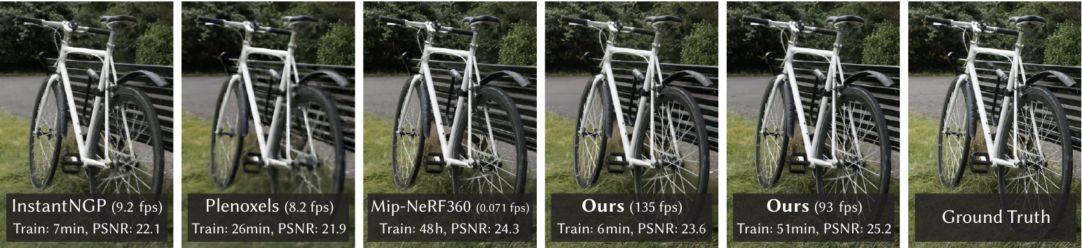
Meshes and points are the most common 3D scene representations because they are explicit and are a good fit for fast GPU/CUDA-based rasterization. In contrast, recent Neural Radiance Field (NeRF) methods build on continuous scene representations, typically optimizing a Multi-Layer Perceptron (MLP) using volumetric ray-marching for novel-view synthesis of captured scenes. Similarly, the most efficient radiance field solutions to date build on continuous representations by interpolating values stored in, e.g., voxel or hash grids or points. While the continuous nature of these methods helps optimization, the stochastic sampling required for rendering is costly and can result in noise. We introduce a new approach that combines the best of both worlds: our 3D Gaussian representation allows optimization with state-of-the-art (SOTA) visual quality and competitive training times, while our tile-based splatting solution ensures real-time rendering at SOTA quality for 1080p resolution on several previously published datasets (see Figure 1).

网格和点是最常见的三维场景表示，因为它们是显式表示，并且非常适合基于 GPU/CUDA 的快速光栅化。 相比之下，近期的神经辐射场（NeRF）方法建立在连续场景表示之上，通常使用体积射线步进优化多层感知机（MLP），以对捕获场景进行新视角合成。 类似地，迄今最高效的辐射场方案也依赖连续表示，通过插值存储在体素网格、哈希网格或点中的数值来工作。 这些方法的连续性质有助于优化，但渲染所需的随机采样代价高昂，并且可能产生噪声。 我们提出一种结合两者优势的新方法：3D 高斯表示能够以先进视觉质量和有竞争力的训练时间完成优化，而基于图块的泼溅方案则能在多个既有数据集上以 1080p 分辨率实现先进质量的实时渲染（见 图1）。

Our goal is to allow real-time rendering for scenes captured with multiple photos, and create the representations with optimization times as fast as the most efficient previous methods for typical real scenes. Recent methods achieve fast training, but struggle to achieve the visual quality obtained by the current SOTA NeRF methods, i.e., Mip-NeRF360, which requires up to 48 hours of training time. The fast -- but lower-quality -- radiance field methods can achieve interactive rendering times depending on the scene (10-15 frames per second), but fall short of real-time rendering at high resolution.

我们的目标是实时渲染由多张照片捕获的场景，并且对于典型真实场景，以媲美既有最高效方法的优化时间构建相应表示。 近期方法能够快速训练，却难以达到当前先进 NeRF 方法 Mip-NeRF360 的视觉质量，而后者需要最长 48 小时的训练时间。 速度较快但质量较低的辐射场方法可根据场景达到交互式渲染速度（每秒 10-15 帧），但在高分辨率下仍达不到实时渲染要求。

Our solution builds on three main components. We first introduce 3D Gaussians as a flexible and expressive scene representation. We start with the same input as previous NeRF-like methods, i.e., cameras calibrated with Structure-from-Motion (SfM) and initialize the set of 3D Gaussians with the sparse point cloud produced for free as part of the SfM process. In contrast to most point-based solutions that require Multi-View Stereo (MVS) data, we achieve high-quality results with only SfM points as input. Note that for the NeRF-synthetic dataset, our method achieves high quality even with random initialization. We show that 3D Gaussians are an excellent choice, since they are a differentiable volumetric representation, but they can also be rasterized very efficiently by projecting them to 2D, and applying standard $\alpha$-blending, using an equivalent image formation model as NeRF. The second component of our method is optimization of the properties of the 3D Gaussians -- 3D position, opacity $\alpha$, anisotropic covariance, and spherical harmonic (SH) coefficients -- interleaved with adaptive density control steps, where we add and occasionally remove 3D Gaussians during optimization. The optimization procedure produces a reasonably compact, unstructured, and precise representation of the scene (1-5 million Gaussians for all scenes tested). The third and final element of our method is our real-time rendering solution that uses fast GPU sorting algorithms and is inspired by tile-based rasterization, following recent work. However, thanks to our 3D Gaussian representation, we can perform anisotropic splatting that respects visibility ordering -- thanks to sorting and $\alpha$-blending -- and enable a fast and accurate backward pass by tracking the traversal of as many sorted splats as required.

我们的方案建立在三个主要组成部分之上。 首先，我们引入 3D 高斯，将其作为灵活且富有表达力的场景表示。 我们采用与既有类 NeRF 方法相同的输入，即由运动恢复结构（SfM）标定的相机，并使用 SfM 过程中自然生成的稀疏点云初始化 3D 高斯集合。 大多数基于点的方案需要多视图立体（MVS）数据，而我们仅以 SfM 点作为输入便能获得高质量结果。 值得注意的是，在 NeRF-synthetic 数据集上，即使使用随机初始化，我们的方法也能获得高质量结果。 我们表明 3D 高斯是一种出色选择：它既是可微体积表示，又可以投影到二维并采用标准 $\alpha$ 混合，以与 NeRF 等价的图像形成模型进行极高效的光栅化。 第二个组成部分是优化 3D 高斯的属性，包括三维位置、不透明度 $\alpha$、各向异性协方差和球谐函数（SH）系数；该过程与自适应密度控制步骤交替执行，在优化期间增加并偶尔移除 3D 高斯。 这一优化过程会产生相当紧凑、非结构化且精确的场景表示（所有测试场景均包含 100 万至 500 万个高斯）。 第三个也是最后一个组成部分，是采用快速 GPU 排序算法并受基于图块的光栅化启发的实时渲染方案。 借助 3D 高斯表示，我们可以通过排序和 $\alpha$ 混合执行遵守可见性顺序的各向异性泼溅，并通过追踪任意所需数量的已排序泼溅基元，实现快速且准确的反向传播。

To summarize, we provide the following contributions:

• The introduction of anisotropic 3D Gaussians as a high-quality, unstructured representation of radiance fields.

• An optimization method of 3D Gaussian properties, interleaved with adaptive density control that creates high-quality representations for captured scenes.

• A fast, differentiable rendering approach for the GPU, which is visibility-aware, allows anisotropic splatting and fast backpropagation to achieve high-quality novel view synthesis.

概括而言，我们作出以下贡献：

• 引入各向异性 3D 高斯，将其作为高质量、非结构化的辐射场表示。

• 提出一种 3D 高斯属性优化方法，并与自适应密度控制交替执行，从而为捕获场景建立高质量表示。

• 提出一种面向 GPU 的快速可微渲染方法；该方法感知可见性，支持各向异性泼溅和快速反向传播，从而实现高质量新视角合成。

Our results on previously published datasets show that we can optimize our 3D Gaussians from multi-view captures and achieve equal or better quality than the best quality previous implicit radiance field approaches. We also can achieve training speeds and quality similar to the fastest methods and importantly provide the first real-time rendering with high quality for novel-view synthesis.

在既有数据集上的结果表明，我们可以从多视图捕获中优化 3D 高斯，并获得不低于既有最高质量隐式辐射场方法的质量。 我们还能够达到与最快方法相近的训练速度和质量，更重要的是首次为新视角合成提供高质量的实时渲染。

2. Related Work

We first briefly overview traditional reconstruction, then discuss point-based rendering and radiance field work, discussing their similarity; radiance fields are a vast area, so we focus only on directly related work. For complete coverage of the field, please see the excellent recent surveys.

我们首先简要回顾传统重建，随后讨论基于点的渲染与辐射场工作以及二者的相似性；辐射场是一个庞大领域，因此这里只关注直接相关的工作。 该领域更完整的梳理可参阅近期的优秀综述。

2.1 Traditional Scene Reconstruction and Rendering

The first novel-view synthesis approaches were based on light fields, first densely sampled then allowing unstructured capture. The advent of Structure-from-Motion (SfM) enabled an entire new domain where a collection of photos could be used to synthesize novel views. SfM estimates a sparse point cloud during camera calibration, that was initially used for simple visualization of 3D space. Subsequent multi-view stereo (MVS) produced impressive full 3D reconstruction algorithms over the years, enabling the development of several view synthesis algorithms. All these methods re-project and blend the input images into the novel view camera, and use the geometry to guide this re-projection. These methods produced excellent results in many cases, but typically cannot completely recover from unreconstructed regions, or from "over-reconstruction", when MVS generates inexistent geometry. Recent neural rendering algorithms vastly reduce such artifacts and avoid the overwhelming cost of storing all input images on the GPU, outperforming these methods on most fronts.

最早的新视角合成方法以光场为基础，起初采用密集采样，之后扩展到非结构化捕获。 运动恢复结构（SfM）的出现开辟了一个全新领域，使人们能够利用一组照片合成新视角。 SfM 在相机标定期间估计稀疏点云，该点云最初用于三维空间的简单可视化。 随后，多视图立体（MVS）在多年发展中产生了令人印象深刻的完整三维重建算法，并推动了多种视角合成算法的发展。 所有这些方法都会把输入图像重投影并混合到新视角相机中，并利用几何引导重投影。 这些方法在许多情况下取得了出色结果，但通常无法完全修复未重建区域，也无法修复 MVS 生成不存在几何时产生的“过度重建”。 近期的神经渲染算法显著减少了这类伪影，并避免在 GPU 上存储所有输入图像的巨大开销，在大多数方面超越了这些方法。

2.2 Neural Rendering and Radiance Fields

Deep learning techniques were adopted early for novel-view synthesis; CNNs were used to estimate blending weights, or for texture-space solutions. The use of MVS-based geometry is a major drawback of most of these methods; in addition, the use of CNNs for final rendering frequently results in temporal flickering.

深度学习技术很早便被用于新视角合成；卷积神经网络被用于估计混合权重或构建纹理空间方案。 大多数此类方法的主要缺点是依赖基于 MVS 的几何；此外，使用卷积神经网络完成最终渲染经常会导致时间闪烁。

Volumetric representations for novel-view synthesis were initiated by Soft3D; deep-learning techniques coupled with volumetric ray-marching were subsequently proposed building on a continuous differentiable density field to represent geometry. Rendering using volumetric ray-marching has a significant cost due to the large number of samples required to query the volume. Neural Radiance Fields (NeRFs) introduced importance sampling and positional encoding to improve quality, but used a large Multi-Layer Perceptron negatively affecting speed. The success of NeRF has resulted in an explosion of follow-up methods that address quality and speed, often by introducing regularization strategies; the current state-of-the-art in image quality for novel-view synthesis is Mip-NeRF360. While the rendering quality is outstanding, training and rendering times remain extremely high; we are able to equal or in some cases surpass this quality while providing fast training and real-time rendering.

Soft3D 开创了面向新视角合成的体积表示；随后，人们提出将深度学习技术与体积射线步进结合，以连续可微密度场表示几何。 由于查询体积需要大量采样，使用体积射线步进进行渲染的成本很高。 神经辐射场（NeRF）引入重要性采样和位置编码来提高质量，但使用了大型多层感知机，因而影响速度。 NeRF 的成功催生了大量旨在改善质量和速度的后续方法，它们通常引入正则化策略；当前新视角合成图像质量的先进方法是 Mip-NeRF360。 尽管其渲染质量出色，训练和渲染时间仍然极高；我们在提供快速训练与实时渲染的同时，可以达到甚至在某些情况下超过这一质量。

The most recent methods have focused on faster training and/or rendering mostly by exploiting three design choices: the use of spatial data structures to store (neural) features that are subsequently interpolated during volumetric ray-marching, different encodings, and MLP capacity. Such methods include different variants of space discretization, codebooks, and encodings such as hash tables, allowing the use of a smaller MLP or foregoing neural networks completely.

最新方法主要利用三种设计选择来加快训练和渲染：使用空间数据结构存储随后在体积射线步进中插值的神经特征、采用不同编码，以及调整 MLP 容量。 这些方法包括不同形式的空间离散化、码本和哈希表等编码，从而能够使用更小的 MLP，甚至完全舍弃神经网络。

Most notable of these methods are InstantNGP which uses a hash grid and an occupancy grid to accelerate computation and a smaller MLP to represent density and appearance; and Plenoxels that use a sparse voxel grid to interpolate a continuous density field, and are able to forgo neural networks altogether. Both rely on Spherical Harmonics: the former to represent directional effects directly, the latter to encode its inputs to the color network. While both provide outstanding results, these methods can still struggle to represent empty space effectively, depending in part on the scene/capture type. In addition, image quality is limited in large part by the choice of the structured grids used for acceleration, and rendering speed is hindered by the need to query many samples for a given ray-marching step. The unstructured, explicit GPU-friendly 3D Gaussians we use achieve faster rendering speed and better quality without neural components.

其中最值得注意的是 InstantNGP 和 Plenoxels：InstantNGP 使用哈希网格与占用网格加速计算，并以较小的 MLP 表示密度和外观；Plenoxels 则使用稀疏体素网格插值连续密度场，因而可以完全舍弃神经网络。 二者都依赖球谐函数：前者用它直接表示方向效应，后者用它编码颜色网络的输入。 尽管两者都取得了出色结果，但根据场景和捕获类型的不同，这些方法仍可能难以有效表示空白空间。 此外，图像质量在很大程度上受用于加速的结构化网格选择限制，而每次射线步进都需要查询大量采样点，也会妨碍渲染速度。 我们采用的非结构化、显式且适合 GPU 的 3D 高斯无需任何神经组件，便能获得更快的渲染速度和更高的质量。

2.3 Point-Based Rendering and Radiance Fields

Point-based methods efficiently render disconnected and unstructured geometry samples (i.e., point clouds). In its simplest form, point sample rendering rasterizes an unstructured set of points with a fixed size, for which it may exploit natively supported point types of graphics APIs or parallel software rasterization on the GPU. While true to the underlying data, point sample rendering suffers from holes, causes aliasing, and is strictly discontinuous. Seminal work on high-quality point-based rendering addresses these issues by "splatting" point primitives with an extent larger than a pixel, e.g., circular or elliptic discs, ellipsoids, or surfels.

基于点的方法能够高效渲染彼此分离且非结构化的几何样本，即点云。 在最简单的形式中，点样本渲染以固定大小光栅化非结构化点集，可以利用图形 API 原生支持的点类型，也可以在 GPU 上进行并行软件光栅化。 尽管忠实于底层数据，点样本渲染仍会产生孔洞和混叠，并且本质上是不连续的。 高质量点渲染的奠基工作通过“泼溅”范围大于一个像素的点基元来解决这些问题，例如圆盘、椭圆盘、椭球体或表面元。

There has been recent interest in differentiable point-based rendering techniques. Points have been augmented with neural features and rendered using a CNN resulting in fast or even real-time view synthesis; however they still depend on MVS for the initial geometry, and as such inherit its artifacts, most notably over- or under-reconstruction in hard cases such as featureless/shiny areas or thin structures.

近期，可微的基于点的渲染技术引起了广泛兴趣。 一些方法为点附加神经特征并使用卷积神经网络渲染，从而实现快速甚至实时的视角合成；但它们仍依赖 MVS 提供初始几何，因此继承了 MVS 的伪影，尤其是在无纹理或光亮区域、细薄结构等困难情况下产生的过度重建或欠重建。

Point-based $\alpha$-blending and NeRF-style volumetric rendering share essentially the same image formation model. Specifically, the color $C$ is given by volumetric rendering along a ray:

基于点的 $\alpha$ 混合与 NeRF 风格的体积渲染本质上共享相同的图像形成模型。 具体而言，颜色 $C$ 由沿射线的体积渲染给出：

$$\begin{array}{}\text{(1)}& \begin{array}{rl}C& =\sum _{i=1}^N{T}_i(1-\exp (-{\sigma }_i{\delta }_i)){\mathbf{c}}_i,\\ T_i& =\exp (-\sum _{j=1}^{i-1}{\sigma }_j{\delta }_j).\end{array}\end{array}$$

Samples of density $\sigma$, transmittance $T$, and color $\mathbf{c}$ are taken along the ray with intervals ${\delta }_i$. This can be re-written as

密度 $\sigma$、透射率 $T$ 和颜色 $\mathbf{c}$ 的样本沿射线以间隔 ${\delta }_i$ 取得。 该式可以改写为

$$\begin{array}{}\text{(2)}& C=\sum _{i=1}^N{T}_i{\alpha }_i{\mathbf{c}}_i,\end{array}$$$$\begin{array}{rl}{\alpha }_i& =1-\exp (-{\sigma }_i{\delta }_i),\\ T_i& =\prod _{j=1}^{i-1}(1-{\alpha }_i).\end{array}$$

A typical neural point-based approach computes the color $C$ of a pixel by blending $\mathcal{N}$ ordered points overlapping the pixel:

典型的神经点渲染方法通过混合覆盖像素的 $\mathcal{N}$ 个有序点来计算像素颜色 $C$：

$$\begin{array}{}\text{(3)}& C=\sum _{i\in \mathcal{N}}{c}_i{\alpha }_i\prod _{j=1}^{i-1}(1-{\alpha }_j),\end{array}$$

Here ${\mathbf{c}}_i$ is the color of each point and ${\alpha }_i$ is given by evaluating a 2D Gaussian with covariance $\mathrm{\Sigma }$ multiplied with a learned per-point opacity. From Equation (2) and Equation (3), we can clearly see that the image formation model is the same. However, the rendering algorithm is very different. NeRFs are a continuous representation implicitly representing empty/occupied space; expensive random sampling is required to find the samples in Equation (2) with consequent noise and computational expense. In contrast, points are an unstructured, discrete representation that is flexible enough to allow creation, destruction, and displacement of geometry similar to NeRF. This is achieved by optimizing opacity and positions, as shown by previous work, while avoiding the shortcomings of a full volumetric representation.

其中，${\mathbf{c}}_i$ 是每个点的颜色，${\alpha }_i$ 由协方差为 $\mathrm{\Sigma }$ 的二维高斯与学习得到的逐点不透明度相乘获得。 从式 (2) 与式 (3) 可以清楚看到，两者的图像形成模型相同。 然而，它们的渲染算法非常不同。 NeRF 是一种隐式表示空白与占用空间的连续表示；为了找到式 (2) 中的样本，需要代价高昂的随机采样，进而带来噪声与计算开销。 相比之下，点是非结构化离散表示，足够灵活，可以像 NeRF 一样创建、销毁和移动几何。 这可以通过优化不透明度和位置实现，同时避开完整体积表示的缺点。

Pulsar achieves fast sphere rasterization which inspired our tile-based and sorting renderer. However, given the analysis above, we want to maintain (approximate) conventional $\alpha$-blending on sorted splats to have the advantages of volumetric representations: Our rasterization respects visibility order in contrast to their order-independent method. In addition, we backpropagate gradients on all splats in a pixel and rasterize anisotropic splats. These elements all contribute to the high visual quality of our results (see Section 7.3). In addition, previous methods mentioned above also use CNNs for rendering, which results in temporal instability. Nonetheless, the rendering speed of Pulsar and ADOP served as motivation to develop our fast rendering solution.

Pulsar 实现了快速的球体光栅化，启发了我们基于图块和排序的渲染器。 然而，基于上述分析，我们希望在已排序泼溅基元上保留近似的传统 $\alpha$ 混合，从而获得体积表示的优势：与其顺序无关方法不同，我们的光栅化遵守可见性顺序。 此外，我们会对一个像素中的所有泼溅基元反向传播梯度，并光栅化各向异性泼溅基元。 这些要素共同促成了结果的高视觉质量（见第 7.3 节）。 另外，上述既有方法也使用卷积神经网络渲染，因而会产生时间不稳定性。 尽管如此，Pulsar 与 ADOP 的渲染速度仍然激励我们开发快速渲染方案。

While focusing on specular effects, the diffuse point-based rendering track of Neural Point Catacaustics overcomes this temporal instability by using an MLP, but still required MVS geometry as input. The most recent method in this category does not require MVS, and also uses SH for directions; however, it can only handle scenes of one object and needs masks for initialization. While fast for small resolutions and low point counts, it is unclear how it can scale to scenes of typical datasets. We use 3D Gaussians for a more flexible scene representation, avoiding the need for MVS geometry and achieving real-time rendering thanks to our tile-based rendering algorithm for the projected Gaussians.

Neural Point Catacaustics 主要关注镜面反射效应，其漫反射点渲染分支通过使用 MLP 克服了时间不稳定性，但仍需要以 MVS 几何作为输入。 该类别中最新的方法不需要 MVS，并且同样使用球谐函数表示方向；然而，它只能处理单个物体的场景，并需要掩码进行初始化。 该方法在低分辨率和少量点时速度很快，但能否扩展到典型数据集中的场景仍不明确。 我们使用 3D 高斯获得更灵活的场景表示，避免对 MVS 几何的需求，并借助针对投影高斯的图块渲染算法实现实时渲染。

A recent approach uses points to represent a radiance field with a radial basis function approach. They employ point pruning and densification techniques during optimization, but use volumetric ray-marching and cannot achieve real-time display rates.

近期有一种方法采用径向基函数，以点来表示辐射场。 该方法在优化期间使用点剪枝与增密技术，但仍采用体积射线步进，无法达到实时显示帧率。

In the domain of human performance capture, 3D Gaussians have been used to represent captured human bodies; more recently they have been used with volumetric ray-marching for vision tasks. Neural volumetric primitives have been proposed in a similar context. While these methods inspired the choice of 3D Gaussians as our scene representation, they focus on the specific case of reconstructing and rendering a single isolated object (a human body or face), resulting in scenes with small depth complexity. In contrast, our optimization of anisotropic covariance, our interleaved optimization/density control, and efficient depth sorting for rendering allow us to handle complete, complex scenes including background, both indoors and outdoors and with large depth complexity.

在人类表演捕获领域，3D 高斯曾被用于表示捕获的人体；近来，它们还与体积射线步进结合用于视觉任务。 类似背景下也有人提出神经体积基元。 这些方法启发我们选择 3D 高斯作为场景表示，但它们聚焦于重建和渲染单个孤立物体（人体或人脸）的特定情况，因此场景的深度复杂度很低。 相比之下，我们对各向异性协方差的优化、交替执行的优化与密度控制，以及渲染时的高效深度排序，使方法能够处理包含背景、横跨室内外且具有高深度复杂度的完整复杂场景。

3. Overview

图2：优化从稀疏 SfM 点云开始并建立 3D 高斯集合，随后优化并自适应控制其密度。快速图块渲染器用于训练和实时场景导航；黑色箭头表示操作流，蓝色箭头表示梯度流。

The input to our method is a set of images of a static scene, together with the corresponding cameras calibrated by SfM which produces a sparse point cloud as a side-effect. From these points we create a set of 3D Gaussians (Section 4), defined by a position (mean), covariance matrix and opacity $\alpha$, that allows a very flexible optimization regime. This results in a reasonably compact representation of the 3D scene, in part because highly anisotropic volumetric splats can be used to represent fine structures compactly. The directional appearance component (color) of the radiance field is represented via spherical harmonics (SH), following standard practice. Our algorithm proceeds to create the radiance field representation (Section 5) via a sequence of optimization steps of 3D Gaussian parameters, i.e., position, covariance, $\alpha$ and SH coefficients interleaved with operations for adaptive control of the Gaussian density. The key to the efficiency of our method is our tile-based rasterizer (Section 6) that allows $\alpha$-blending of anisotropic splats, respecting visibility order thanks to fast sorting. Our fast rasterizer also includes a fast backward pass by tracking accumulated $\alpha$ values, without a limit on the number of Gaussians that can receive gradients. The overview of our method is illustrated in Figure 2.

我们的方法以静态场景的一组图像及其经 SfM 标定的相机为输入，SfM 还会附带产生一个稀疏点云。 我们从这些点建立一组 3D 高斯（第 4 节），每个高斯由位置（均值）、协方差矩阵和不透明度 $\alpha$ 定义，从而支持非常灵活的优化过程。 这会产生相当紧凑的三维场景表示，部分原因在于高度各向异性的体积泼溅基元能够紧凑表示精细结构。 按照标准做法，辐射场的方向相关外观分量（颜色）由球谐函数（SH）表示。 算法通过一系列 3D 高斯参数优化步骤建立辐射场表示（第 5 节），即交替优化位置、协方差、$\alpha$ 和 SH 系数，并执行自适应高斯密度控制操作。 方法高效性的关键是基于图块的光栅器（第 6 节）：它支持各向异性泼溅基元的 $\alpha$ 混合，并借助快速排序遵守可见性顺序。 我们的快速光栅器还通过追踪累积 $\alpha$ 值实现快速反向传播，并且不限制能够接收梯度的高斯数量。 方法总览如 图2 所示。

4. Differentiable 3D Gaussian Splatting

Our goal is to optimize a scene representation that allows high-quality novel view synthesis, starting from a sparse set of (SfM) points without normals. To do this, we need a primitive that inherits the properties of differentiable volumetric representations, while at the same time being unstructured and explicit to allow very fast rendering. We choose 3D Gaussians, which are differentiable and can be easily projected to 2D splats allowing fast $\alpha$-blending for rendering.

我们的目标是从一组不带法线的稀疏 SfM 点出发，优化一种支持高质量新视角合成的场景表示。 为此，我们需要一种继承可微体积表示性质，同时保持非结构化和显式特征以支持极快渲染的基元。 我们选择 3D 高斯；它既可微，又能方便地投影为二维泼溅基元，通过快速 $\alpha$ 混合完成渲染。

Our representation has similarities to previous methods that use 2D points and assume each point is a small planar circle with a normal. Given the extreme sparsity of SfM points it is very hard to estimate normals. Similarly, optimizing very noisy normals from such an estimation would be very challenging. Instead, we model the geometry as a set of 3D Gaussians that do not require normals. Our Gaussians are defined by a full 3D covariance matrix $\mathrm{\Sigma }$ defined in world space centered at point (mean) $\mu$:

我们的表示与既有二维点方法相似，后者假设每个点都是带法线的小型平面圆盘。 由于 SfM 点极其稀疏，估计法线非常困难。 同样，从这种估计中优化噪声很大的法线也非常具有挑战性。 因此，我们把几何建模为一组不需要法线的 3D 高斯。 高斯由定义在世界空间、以点（均值）$\mu$ 为中心的完整三维协方差矩阵 $\mathrm{\Sigma }$ 定义：

$$\begin{array}{}\text{(4)}& G(x)=\exp (-\frac{1}{2}{x}^T{\mathrm{\Sigma }}^{-1}x).\end{array}$$

This Gaussian is multiplied by $\alpha$ in our blending process. However, we need to project our 3D Gaussians to 2D for rendering. Zwicker et al. demonstrate how to do this projection to image space. Given a viewing transformation $W$ the covariance matrix ${\mathrm{\Sigma }}^{\prime }$ in camera coordinates is given as follows:

在混合过程中，该高斯会乘以 $\alpha$。 然而，为了进行渲染，我们需要把 3D 高斯投影到二维空间。 Zwicker 等人给出了这种图像空间投影的方法。 给定视图变换 $W$，相机坐标下的协方差矩阵 ${\mathrm{\Sigma }}^{\prime }$ 如下：

$$\begin{array}{}\text{(5)}& {\mathrm{\Sigma }}^{\prime }=JW\mathrm{\Sigma }{W}^T{J}^T.\end{array}$$

Here $J$ is the Jacobian of the affine approximation of the projective transformation. Zwicker et al. also show that if we skip the third row and column of ${\mathrm{\Sigma }}^{\prime }$, we obtain a $2\times 2$ variance matrix with the same structure and properties as if we would start from planar points with normals, as in previous work.

其中，$J$ 是投影变换仿射近似的雅可比矩阵。 Zwicker 等人还表明，如果舍弃 ${\mathrm{\Sigma }}^{\prime }$ 的第三行和第三列，便会得到一个 $2\times 2$ 方差矩阵，其结构和性质与从带法线平面点出发的既有方法相同。

An obvious approach would be to directly optimize the covariance matrix $\mathrm{\Sigma }$ to obtain 3D Gaussians that represent the radiance field. However, covariance matrices have physical meaning only when they are positive semi-definite. For our optimization of all our parameters, we use gradient descent that cannot be easily constrained to produce such valid matrices, and update steps and gradients can very easily create invalid covariance matrices.

一种直观做法是直接优化协方差矩阵 $\mathrm{\Sigma }$，得到表示辐射场的 3D 高斯。 然而，协方差矩阵只有在半正定时才具有物理意义。 我们使用梯度下降优化所有参数，但很难约束它始终产生有效矩阵，更新步骤和梯度也很容易生成无效协方差矩阵。

As a result, we opted for a more intuitive, yet equivalently expressive representation for optimization. The covariance matrix $\mathrm{\Sigma }$ of a 3D Gaussian is analogous to describing the configuration of an ellipsoid. Given a scaling matrix $S$ and rotation matrix $R$, we can find the corresponding $\mathrm{\Sigma }$:

因此，我们选择一种更直观但表达能力等价的优化表示。 3D 高斯的协方差矩阵 $\mathrm{\Sigma }$ 类似于对椭球体构型的描述。 给定缩放矩阵 $S$ 和旋转矩阵 $R$，可以得到相应的 $\mathrm{\Sigma }$：

$$\begin{array}{}\text{(6)}& \mathrm{\Sigma }=RS{S}^T{R}^T.\end{array}$$

To allow independent optimization of both factors, we store them separately: a 3D vector $s$ for scaling and a quaternion $q$ to represent rotation. These can be trivially converted to their respective matrices and combined, making sure to normalize $q$ to obtain a valid unit quaternion. To avoid significant overhead due to automatic differentiation during training, we derive the gradients for all parameters explicitly. Details of the exact derivative computations are in the appendix. This representation of anisotropic covariance -- suitable for optimization -- allows us to optimize 3D Gaussians to adapt to the geometry of different shapes in captured scenes, resulting in a fairly compact representation. Figure 3 illustrates such cases.

为了独立优化两个因子，我们分别存储它们：三维向量 $s$ 表示缩放，四元数 $q$ 表示旋转。 二者可以直接转换成各自矩阵并组合，同时对 $q$ 进行归一化以获得有效的单位四元数。 为了避免训练期间自动微分带来的巨大开销，我们显式推导所有参数的梯度。 精确的导数计算细节见附录。 这种适合优化的各向异性协方差表示，使我们能够优化 3D 高斯以适应捕获场景中不同形状的几何，从而得到相当紧凑的表示。 图3 展示了这类情况。

图3：将优化后的 3D 高斯缩小 60% 进行可视化（最右），可以清楚看到各向异性形状如何紧凑表示复杂几何；左侧为实际渲染图像。

5. Optimization with Adaptive Density Control of 3D Gaussians

The core of our approach is the optimization step, which creates a dense set of 3D Gaussians accurately representing the scene for free-view synthesis. In addition to positions $p$, $\alpha$, and covariance $\mathrm{\Sigma }$, we also optimize SH coefficients representing color $c$ of each Gaussian to correctly capture the view-dependent appearance of the scene. The optimization of these parameters is interleaved with steps that control the density of the Gaussians to better represent the scene.

我们方法的核心是优化步骤，它建立一组能够准确表示场景的稠密 3D 高斯，用于自由视角合成。 除位置 $p$、$\alpha$ 和协方差 $\mathrm{\Sigma }$ 外，我们还优化表示每个高斯颜色 $c$ 的 SH 系数，以正确捕获场景的视角相关外观。 这些参数的优化与高斯密度控制步骤交替执行，从而更好地表示场景。

5.1 Optimization

The optimization is based on successive iterations of rendering and comparing the resulting image to the training views in the captured dataset. Inevitably, geometry may be incorrectly placed due to the ambiguities of 3D to 2D projection. Our optimization thus needs to be able to create geometry and also destroy or move geometry if it has been incorrectly positioned. The quality of the parameters of the covariances of the 3D Gaussians is critical for the compactness of the representation since large homogeneous areas can be captured with a small number of large anisotropic Gaussians.

优化通过反复渲染，并将生成图像与捕获数据集中的训练视图比较来进行。 由于三维到二维投影存在歧义，几何不可避免地可能被放置在错误位置。 因此，优化过程必须能够创建几何，也要能在几何位置错误时将其销毁或移动。 3D 高斯协方差参数的质量对表示紧凑性至关重要，因为只需少量大型各向异性高斯便能捕获大面积均匀区域。

We use Stochastic Gradient Descent techniques for optimization, taking full advantage of standard GPU-accelerated frameworks, and the ability to add custom CUDA kernels for some operations, following recent best practice. In particular, our fast rasterization (see Section 6) is critical in the efficiency of our optimization, since it is the main computational bottleneck of the optimization. We use a sigmoid activation function for $\alpha$ to constrain it in the $[0,1)$ range and obtain smooth gradients, and an exponential activation function for the scale of the covariance for similar reasons.

我们使用随机梯度下降技术进行优化，充分利用标准 GPU 加速框架，并遵循近期最佳实践，为部分操作添加自定义 CUDA kernel。 尤其是快速光栅化（见第 6 节）对优化效率至关重要，因为它是优化的主要计算瓶颈。 我们对 $\alpha$ 使用 sigmoid 激活函数，将其约束在 $[0,1)$ 范围内并获得平滑梯度；出于类似原因，对协方差的尺度使用指数激活函数。

We estimate the initial covariance matrix as an isotropic Gaussian with axes equal to the mean of the distance to the closest three points. We use a standard exponential decay scheduling technique similar to Plenoxels, but for positions only. The loss function is ${\mathcal{L}}_1$ combined with a D-SSIM term:

我们把初始协方差矩阵估计为各向同性高斯，其各轴长度等于到最近三个点距离的均值。 我们采用与 Plenoxels 类似的标准指数衰减调度技术，但只将其用于位置。 损失函数由 ${\mathcal{L}}_1$ 与 D-SSIM 项组合而成：

$$\begin{array}{}\text{(7)}& \mathcal{L}=(1-\lambda ){\mathcal{L}}_1+\lambda {\mathcal{L}}_{\mathrm{D}\text{-}\mathrm{SSIM}}.\end{array}$$

We use $\lambda =0.2$ in all our tests. We provide details of the learning schedule and other elements in Section 7.1.

所有测试均使用 $\lambda =0.2$。 学习调度与其他要素的细节见第 7.1 节。

5.2 Adaptive Control of Gaussians

We start with the initial set of sparse points from SfM and then apply our method to adaptively control the number of Gaussians and their density over unit volume, allowing us to go from an initial sparse set of Gaussians to a denser set that better represents the scene, and with correct parameters. Density of Gaussians should not be confused of course with density $\sigma$ in the NeRF literature. After optimization warm-up (see Section 7.1), we densify every 100 iterations and remove any Gaussians that are essentially transparent, i.e., with $\alpha$ less than a threshold ${ϵ}_{\alpha }$.

我们从 SfM 的初始稀疏点集出发，自适应控制高斯数量及其单位体积密度，从而把初始稀疏高斯集转变为参数正确、能够更好表示场景的稠密集合。 当然，高斯密度不应与 NeRF 文献中的密度 $\sigma$ 混淆。 优化预热后（见第 7.1 节），我们每 100 次迭代执行一次增密，并移除基本透明的高斯，即 $\alpha$ 小于阈值 ${ϵ}_{\alpha }$ 的高斯。

Our adaptive control of the Gaussians needs to populate empty areas. It focuses on regions with missing geometric features ("under-reconstruction"), but also in regions where Gaussians cover large areas in the scene (which often correspond to "over-reconstruction"). We observe that both have large view-space positional gradients. Intuitively, this is likely because they correspond to regions that are not yet well reconstructed, and the optimization tries to move the Gaussians to correct this. Since both cases are good candidates for densification, we densify Gaussians with an average magnitude of view-space position gradients above a threshold ${\tau }_{\mathrm{pos}}$, which we set to $0.0002$ in our tests. We next present details of this process, illustrated in Figure 4.

高斯的自适应控制需要填充空白区域。 它既关注缺少几何特征的区域，即“欠重建”区域，也关注高斯覆盖场景中大面积范围的区域，这通常对应“过度重建”。 我们观察到，两类区域都具有较大的视图空间位置梯度。 直观而言，这可能是因为它们对应尚未得到良好重建的区域，而优化会尝试移动高斯进行修正。 由于两种情况都适合增密，我们对视图空间位置梯度平均幅值高于阈值 ${\tau }_{\mathrm{pos}}$ 的高斯执行增密，并在测试中将该阈值设为 $0.0002$。 该过程的细节如 图4 所示。

图4：自适应高斯增密方案。上排（欠重建）：小尺度几何覆盖不足时，克隆相应高斯。下排（过度重建）：一个大型泼溅基元表示小尺度几何时，将其拆分为两个。

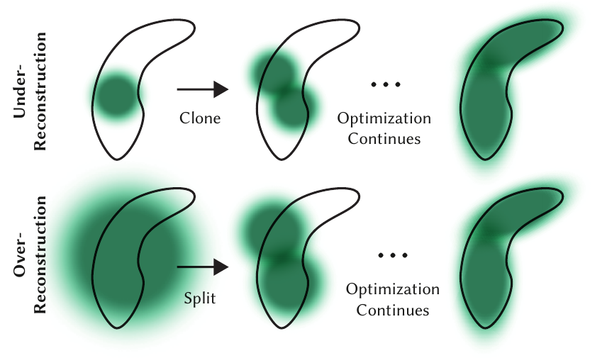
For small Gaussians that are in under-reconstructed regions, we need to cover the new geometry that must be created. For this, it is preferable to clone the Gaussians, by simply creating a copy of the same size, and moving it in the direction of the positional gradient. On the other hand, large Gaussians in regions with high variance need to be split into smaller Gaussians. We replace such Gaussians by two new ones, and divide their scale by a factor of $\varphi =1.6$ which we determined experimentally. We also initialize their position by using the original 3D Gaussian as a PDF for sampling.

对于位于欠重建区域的小型高斯，我们需要覆盖必须新建的几何。 为此，更合适的做法是克隆高斯：直接建立一个大小相同的副本，并沿位置梯度方向移动它。 另一方面，高方差区域中的大型高斯需要拆分成较小高斯。 我们用两个新高斯替换这类高斯，并把尺度除以通过实验确定的因子 $\varphi =1.6$。 我们还把原始 3D 高斯作为概率密度函数进行采样，以初始化新高斯的位置。

In the first case we detect and treat the need for increasing both the total volume of the system and the number of Gaussians, while in the second case we conserve total volume but increase the number of Gaussians. Similar to other volumetric representations, our optimization can get stuck with floaters close to the input cameras; in our case this may result in an unjustified increase in the Gaussian density. An effective way to moderate the increase in the number of Gaussians and to deal with the floaters is to set the $\alpha$ value close to zero every $N=3000$ iterations. The optimization then increases the $\alpha$ for the Gaussians where this is needed while allowing our culling approach to remove Gaussians with $\alpha$ less than ${ϵ}_{\alpha }$ as described above. Gaussians may shrink or grow and considerably overlap with others, but we periodically remove Gaussians that are very large in worldspace and those that have a big footprint in viewspace. This strategy results in overall good control over the total number of Gaussians. The Gaussians in our model remain primitives in Euclidean space at all times; unlike other methods, we do not require space compaction, warping or projection strategies for distant or large Gaussians.

在第一种情况下，我们检测并处理同时增加系统总体积与高斯数量的需求；在第二种情况下，则保持总体积不变但增加高斯数量。 与其他体积表示类似，我们的优化可能困在输入相机附近的漂浮伪影中；在本方法中，这可能导致高斯密度无正当理由地增加。 一种有效抑制高斯数量增长并处理漂浮伪影的方法，是每隔 $N=3000$ 次迭代把 $\alpha$ 值重置到接近零。 随后，优化会在需要的高斯上增大 $\alpha$，同时允许上述剔除方法移除 $\alpha$ 小于 ${ϵ}_{\alpha }$ 的高斯。 高斯可能缩小或增大，并与其他高斯大幅重叠；但我们会周期性移除世界空间中尺寸很大，以及视图空间中覆盖范围很大的高斯。 该策略使高斯总数整体上得到良好控制。 模型中的高斯始终是欧氏空间中的基元；与其他方法不同，我们无需针对远距离或大型高斯采用空间压缩、扭曲或投影策略。

6. Fast Differentiable Rasterizer for Gaussians

Our goals are to have fast overall rendering and fast sorting to allow approximate $\alpha$-blending -- including for anisotropic splats -- and to avoid hard limits on the number of splats that can receive gradients that exist in previous work.

我们的目标是通过快速整体渲染和快速排序，支持包括各向异性泼溅在内的近似 $\alpha$ 混合，并避免既有工作中对可接收梯度的泼溅基元数量所施加的硬性限制。

To achieve these goals, we design a tile-based rasterizer for Gaussian splats inspired by recent software rasterization approaches to pre-sort primitives for an entire image at a time, avoiding the expense of sorting per pixel that hindered previous $\alpha$-blending solutions. Our fast rasterizer allows efficient backpropagation over an arbitrary number of blended Gaussians with low additional memory consumption, requiring only a constant overhead per pixel. Our rasterization pipeline is fully differentiable, and given the projection to 2D (Section 4) can rasterize anisotropic splats similar to previous 2D splatting methods.

为了实现这些目标，我们受近期软件光栅化方法启发，为高斯泼溅设计了基于图块的光栅器；它一次性为整幅图像预排序基元，避免既有 $\alpha$ 混合方案中逐像素排序的高昂成本。 快速光栅器仅需每像素恒定的额外开销和少量附加内存，就能对任意数量的混合高斯高效反向传播。 整个光栅化管线完全可微，并可根据二维投影（第 4 节），像既有二维泼溅方法一样光栅化各向异性泼溅基元。

Our method starts by splitting the screen into $16\times 16$ tiles, and then proceeds to cull 3D Gaussians against the view frustum and each tile. Specifically, we only keep Gaussians with a 99% confidence interval intersecting the view frustum. Additionally, we use a guard band to trivially reject Gaussians at extreme positions (i.e., those with means close to the near plane and far outside the view frustum), since computing their projected 2D covariance would be unstable. We then instantiate each Gaussian according to the number of tiles they overlap and assign each instance a key that combines view space depth and tile ID. We then sort Gaussians based on these keys using a single fast GPU Radix sort. Note that there is no additional per-pixel ordering of points, and blending is performed based on this initial sorting. As a consequence, our $\alpha$-blending can be approximate in some configurations. However, these approximations become negligible as splats approach the size of individual pixels. We found that this choice greatly enhances training and rendering performance without producing visible artifacts in converged scenes.

我们首先把屏幕划分成 $16\times 16$ 图块，随后针对视锥体和每个图块剔除 3D 高斯。 具体而言，只保留 99% 置信区间与视锥体相交的高斯。 此外，我们使用保护带直接拒绝位于极端位置的高斯，即均值靠近近裁剪面且远在视锥体外的高斯，因为计算它们投影后的二维协方差会不稳定。 随后，根据每个高斯重叠的图块数量将其实例化，并为每个实例分配一个结合视图空间深度和图块 ID 的键。 我们使用一次快速 GPU 基数排序，依据这些键对高斯排序。 需要注意的是，这里不再进行额外的逐像素点排序，混合完全依据初始排序执行。 因此，在某些配置下，$\alpha$ 混合可能只是近似的。 不过，当泼溅基元接近单个像素大小时，这种近似可以忽略不计。 我们发现，该选择显著提高了训练和渲染性能，同时不会在收敛场景中产生可见伪影。

After sorting Gaussians, we produce a list for each tile by identifying the first and last depth-sorted entry that splats to a given tile. For rasterization, we launch one thread block for each tile. Each block first collaboratively loads packets of Gaussians into shared memory and then, for a given pixel, accumulates color and $\alpha$ values by traversing the lists front-to-back, thus maximizing the gain in parallelism both for data loading/sharing and processing. When we reach a target saturation of $\alpha$ in a pixel, the corresponding thread stops. At regular intervals, threads in a tile are queried and the processing of the entire tile terminates when all pixels have saturated (i.e., $\alpha$ goes to 1). Details of sorting and a high-level overview of the overall rasterization approach are given in the appendix.

高斯排序后，我们通过确定泼溅到指定图块的首个和末个深度排序条目，为每个图块生成列表。 光栅化时，每个图块启动一个线程块。 每个线程块首先协作地把成批高斯加载到共享内存中；随后针对给定像素从前到后遍历列表，累积颜色和 $\alpha$ 值，从而在数据加载、共享和处理两方面最大化并行收益。 当像素中的 $\alpha$ 达到目标饱和度时，相应线程停止。 系统定期查询图块内的线程；当所有像素都已饱和，即 $\alpha$ 趋近于 1 时，整个图块停止处理。 排序细节和整体光栅化方法的高层概览见附录。

During rasterization, the saturation of $\alpha$ is the only stopping criterion. In contrast to previous work, we do not limit the number of blended primitives that receive gradient updates. We enforce this property to allow our approach to handle scenes with an arbitrary, varying depth complexity and accurately learn them, without having to resort to scene-specific hyperparameter tuning. During the backward pass, we must therefore recover the full sequence of blended points per-pixel in the forward pass. One solution would be to store arbitrarily long lists of blended points per-pixel in global memory. To avoid the implied dynamic memory management overhead, we instead choose to traverse the per-tile lists again; we can reuse the sorted array of Gaussians and tile ranges from the forward pass. To facilitate gradient computation, we now traverse them back-to-front.

在光栅化期间，$\alpha$ 饱和是唯一的停止条件。 与既有工作不同，我们不限制接收梯度更新的混合基元数量。 这一性质使方法能够处理并准确学习具有任意且变化深度复杂度的场景，而无需针对具体场景调整超参数。 因此，在反向传播期间，我们必须恢复前向传播中每个像素的完整混合点序列。 一种方案是在全局内存中存储每像素任意长度的混合点列表。 为避免由此产生的动态内存管理开销，我们选择再次遍历逐图块列表，并复用前向传播中的已排序高斯数组和图块范围。 为了便于计算梯度，此时按从后到前的顺序遍历。

The traversal starts from the last point that affected any pixel in the tile, and loading of points into shared memory again happens collaboratively. Additionally, each pixel will only start (expensive) overlap testing and processing of points if their depth is lower than or equal to the depth of the last point that contributed to its color during the forward pass. Computation of the gradients described in Section 4 requires the accumulated opacity values at each step during the original blending process. Rather than traversing an explicit list of progressively shrinking opacities in the backward pass, we can recover these intermediate opacities by storing only the total accumulated opacity at the end of the forward pass. Specifically, each point stores the final accumulated opacity $\alpha$ in the forward process; we divide this by each point's $\alpha$ in our back-to-front traversal to obtain the required coefficients for gradient computation.

遍历从影响图块中任意像素的最后一个点开始，并再次协作地将点加载到共享内存。 此外，仅当点的深度小于或等于前向传播中最后一个对像素颜色有贡献的点的深度时，每个像素才会开始代价较高的重叠测试和点处理。 计算第 4 节所述梯度，需要原始混合过程每一步的累积不透明度值。 与其在反向传播中遍历逐渐减小的不透明度显式列表，我们只存储前向传播结束时的总累积不透明度，就能恢复这些中间不透明度。 具体而言，每个点在前向过程中存储最终累积不透明度 $\alpha$；在从后到前遍历时，将它除以每个点自身的 $\alpha$，便可得到梯度计算所需的系数。

图5：我们将该方法与既有方法及其在留出测试视角上的对应真实图像进行比较。场景从上到下依次为：Mip-NeRF360 数据集中的 Bicycle、Garden、Stump、Counter 和 Room；Deep Blending 数据集中的 Playroom、DrJohnson；以及 Tanks&Temples 中的 Truck 和 Train。箭头或局部放大框突出显示了不易察觉的质量差异。

表1：在三个数据集上对该方法与既有工作的定量比较。带 † 的结果直接取自原论文，其余结果均来自我们的实验。

Method	Mip-NeRF360						Tanks&Temples						Deep Blending
	SSIM↑	PSNR↑	LPIPS↓	Train	FPS	Mem	SSIM↑	PSNR↑	LPIPS↓	Train	FPS	Mem	SSIM↑	PSNR↑	LPIPS↓	Train	FPS	Mem
Plenoxels	0.626	23.08	0.463	25m49s	6.79	2.1GB	0.719	21.08	0.379	25m5s	13.0	2.3GB	0.795	23.06	0.510	27m49s	11.2	2.7GB
INGP-Base	0.671	25.30	0.371	5m37s	11.7	13MB	0.723	21.72	0.330	5m26s	17.1	13MB	0.797	23.62	0.423	6m31s	3.26	13MB
INGP-Big	0.699	25.59	0.331	7m30s	9.43	48MB	0.745	21.92	0.305	6m59s	14.4	48MB	0.817	24.96	0.390	8m	2.79	48MB
M-NeRF360	0.792†	27.69†	0.237†	48h	0.06	8.6MB	0.759	22.22	0.257	48h	0.14	8.6MB	0.901	29.40	0.245	48h	0.09	8.6MB
Ours-7K	0.770	25.60	0.279	6m25s	160	523MB	0.767	21.20	0.280	6m55s	197	270MB	0.875	27.78	0.317	4m35s	172	386MB
Ours-30K	0.815	27.21	0.214	41m33s	134	734MB	0.841	23.14	0.183	26m54s	154	411MB	0.903	29.41	0.243	36m2s	137	676MB

图6：对于部分场景（上），即使只训练 7K 次迭代（该场景约 5 分钟），我们的方法也已很好地捕获列车；训练至 30K 次迭代（约 35 分钟）后，背景伪影显著减少。对于另一些场景（下），差异几乎不可见，7K 次迭代（约 8 分钟）便已达到很高质量。

7. Implementation, Results and Evaluation

We next discuss some details of implementation, present results and the evaluation of our algorithm compared to previous work and ablation studies.

下面，我们讨论实现细节，给出实验结果，并通过与既有工作比较及消融研究来评估算法。

表2：Synthetic NeRF 上的 PSNR 分数；我们从 100K 个随机初始化点开始训练。竞争方法的指标取自各自论文。

Method	Mic	Chair	Ship	Materials	Lego	Drums	Ficus	Hotdog	Avg.
Plenoxels	33.26	33.98	29.62	29.14	34.10	25.35	31.83	36.81	31.76
INGP-Base	36.22	35.00	31.10	29.78	36.39	26.02	33.51	37.40	33.18
Mip-NeRF	36.51	35.14	30.41	30.71	35.70	25.48	33.29	37.48	33.09
Point-NeRF	35.95	35.40	30.97	29.61	35.04	26.06	36.13	37.30	33.30
Ours-30K	35.36	35.83	30.80	30.00	35.78	26.15	34.87	37.72	33.32

7.1 Implementation

We implemented our method in Python using the PyTorch framework and wrote custom CUDA kernels for rasterization that are extended versions of previous methods, and use the NVIDIA CUB sorting routines for the fast Radix sort. We also built an interactive viewer using the open-source SIBR, used for interactive viewing. We used this implementation to measure our achieved frame rates. The source code and all our data are available at: https://repo-sam.inria.fr/fungraph/3d-gaussian-splatting/.

我们使用 PyTorch 框架以 Python 实现该方法，并为光栅化编写了由既有方法扩展而来的自定义 CUDA 核函数，同时使用 NVIDIA CUB 排序例程执行快速基数排序。 我们还使用开源 SIBR 构建了用于交互查看的交互式查看器。 我们使用该实现测量所达到的帧率。 源代码和全部数据见：https://repo-sam.inria.fr/fungraph/3d-gaussian-splatting/。

Optimization Details. For stability, we "warm-up" the computation in lower resolution. Specifically, we start the optimization using 4 times smaller image resolution and we upsample twice after 250 and 500 iterations.

优化细节。 为提高稳定性，我们先在较低分辨率下对计算进行“预热”。 具体而言，优化从缩小 4 倍的图像分辨率开始，并分别在 250 次和 500 次迭代后进行两次上采样。

SH coefficient optimization is sensitive to the lack of angular information. For typical "NeRF-like" captures where a central object is observed by photos taken in the entire hemisphere around it, the optimization works well. However, if the capture has angular regions missing (e.g., when capturing the corner of a scene, or performing an "inside-out" capture) completely incorrect values for the zero-order component of the SH (i.e., the base or diffuse color) can be produced by the optimization. To overcome this problem we start by optimizing only the zero-order component, and then introduce one band of the SH after every 1000 iterations until all 4 bands of SH are represented.

球谐函数（SH）系数优化对角度信息缺失较为敏感。 对于典型的“NeRF 式”捕获，即从中心物体周围整个半球拍摄照片，优化效果良好。 然而，如果捕获数据缺少某些角度区域，例如拍摄场景角落或执行“由内向外”捕获，优化可能为 SH 的零阶分量，即基础色或漫反射颜色，生成完全错误的值。 为解决该问题，我们一开始只优化零阶分量，随后每隔 1000 次迭代引入一个 SH 频带，直至表示全部 4 个频带。

表3：消融实验的 PSNR 分数。该实验将各场景的高分辨率输入图像手动降采样到其他实验采用的既定渲染分辨率，从而减少随机伪影，例如预先缩小的 Mip-NeRF360 输入中的 JPEG 压缩伪影。

Variant	Truck-5K	Garden-5K	Bicycle-5K	Truck-30K	Garden-30K	Bicycle-30K	Average-5K	Average-30K
Limited-BW	14.66	22.07	20.77	13.84	22.88	20.87	19.16	19.19
Random Init	16.75	20.90	19.86	18.02	22.19	21.05	19.17	20.42
No-Split	18.31	23.98	22.21	20.59	26.11	25.02	21.50	23.90
No-SH	22.36	25.22	22.88	24.39	26.59	25.08	23.48	25.35
No-Clone	22.29	25.61	22.15	24.82	27.47	25.46	23.35	25.91
Isotropic	22.40	25.49	22.81	23.89	27.00	24.81	23.56	25.23
Full	22.71	25.82	23.18	24.81	27.70	25.65	23.90	26.05

7.2 Results and Evaluation

Results. We tested our algorithm on a total of 13 real scenes taken from previously published datasets and the synthetic Blender dataset. In particular, we tested our approach on the full set of scenes presented in Mip-Nerf360, which is the current state of the art in NeRF rendering quality, two scenes from the Tanks&Temples dataset and two scenes provided by Hedman et al. The scenes we chose have very different capture styles, and cover both bounded indoor scenes and large unbounded outdoor environments. We use the same hyperparameter configuration for all experiments in our evaluation. All results are reported running on an A6000 GPU, except for the Mip-NeRF360 method (see below).

结果。 我们在既有公开数据集的 13 个真实场景以及合成 Blender 数据集上测试了算法。 具体而言，我们在 Mip-NeRF360 给出的全部场景、Tanks&Temples 数据集的两个场景，以及 Hedman 等人提供的两个场景上进行了测试；Mip-NeRF360 是当时 NeRF 渲染质量的先进方法。 所选场景具有截然不同的捕获方式，既包括有边界的室内场景，也包括大型无边界室外环境。 评估中的所有实验均采用相同的超参数配置。 除下文说明的 Mip-NeRF360 方法外，所有结果均在 A6000 GPU 上运行得到。

In supplemental, we show a rendered video path for a selection of scenes that contain views far from the input photos.

补充材料展示了若干场景的渲染视频路径，其中包含远离输入照片视角的视图。

Real-World Scenes. In terms of quality, the current state-of-the-art is Mip-Nerf360. We compare against this method as a quality benchmark. We also compare against two of the most recent fast NeRF methods: InstantNGP and Plenoxels.

真实场景。 就质量而言，当时的先进方法是 Mip-NeRF360。 我们将该方法作为质量基准进行比较。 我们还与两个近期快速 NeRF 方法 InstantNGP 和 Plenoxels 进行比较。

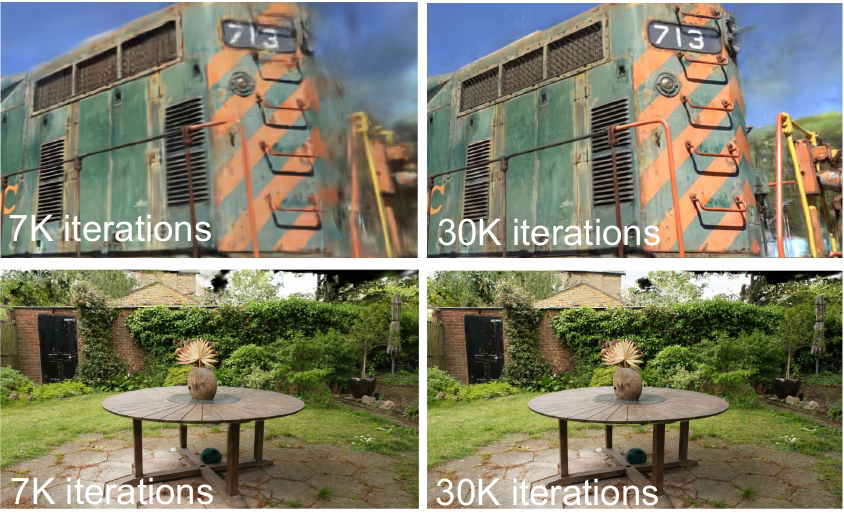
We use a train/test split for datasets, using the methodology suggested by Mip-NeRF360, taking every 8th photo for test, for consistent and meaningful comparisons to generate the error metrics, using the standard PSNR, L-PIPS, and SSIM metrics used most frequently in the literature; please see Table 1. All numbers in the table are from our own runs of the author's code for all previous methods, except for those of Mip-NeRF360 on their dataset, in which we copied the numbers from the original publication to avoid confusion about the current SOTA. For the images in our figures, we used our own run of Mip-NeRF360: the numbers for these runs are in Appendix. We also show the average training time, rendering speed, and memory used to store optimized parameters. We report results for a basic configuration of InstantNGP (Base) that run for 35K iterations as well as a slightly larger network suggested by the authors (Big), and two configurations, 7K and 30K iterations for ours. We show the difference in visual quality for our two configurations in Figure 6. In many cases, quality at 7K iterations is already quite good.

我们按照 Mip-NeRF360 建议的方法划分数据集的训练集和测试集，每隔 8 张照片取一张作为测试图像，以生成一致且有意义的误差指标比较；采用文献中最常用的标准 PSNR、L-PIPS 和 SSIM 指标，见 表1。 表中的数字均来自我们运行各既有方法作者代码所得的结果，只有 Mip-NeRF360 在其自身数据集上的结果直接取自原论文，以免对当时的先进水平造成混淆。 图中使用的是我们自行运行 Mip-NeRF360 得到的图像，相应数值见附录。 我们还报告平均训练时间、渲染速度，以及存储优化参数所需的内存。 InstantNGP 报告运行 35K 次迭代的基础配置（Base）和作者建议的稍大网络（Big）；我们的方法则报告 7K 和 30K 次迭代两个配置。 两个配置的视觉质量差异见 图6。 在许多情况下，7K 次迭代的质量已经相当出色。

The training times vary over datasets and we report them separately. Note that image resolutions also vary over datasets. In the project website, we provide all the renders of test views we used to compute the statistics for all the methods (ours and previous work) on all scenes. Note that we kept the native input resolution for all renders.

训练时间因数据集而异，因此分别报告。 图像分辨率同样因数据集而异。 项目网站提供了所有场景上用于计算各方法统计数据的全部测试视角渲染结果，包括我们的方法和既有工作。 所有渲染均保留原生输入分辨率。

The table shows that our fully converged model achieves quality that is on par and sometimes slightly better than the SOTA Mip-NeRF360 method; note that on the same hardware, their average training time was 48 hours, compared to our 35-45min, and their rendering time is 10s/frame. We trained Mip-NeRF360 on a 4-GPU A100 node for 12 hours, equivalent to 48 hours on a single GPU. Note that A100's are faster than A6000 GPUs. We achieve comparable quality to InstantNGP and Plenoxels after 5-10m of training, but additional training time allows us to achieve SOTA quality which is not the case for the other fast methods. For Tanks & Temples, we achieve similar quality as the basic InstantNGP at a similar training time ($\sim$ 7min in our case).

表中显示，完全收敛的模型质量与先进的 Mip-NeRF360 相当，有时还略胜一筹；需要注意的是，在相同硬件上，后者平均需要训练 48 小时，而我们仅需 35–45 分钟，且其渲染时间为每帧 10 秒。 我们在配备 4 块 A100 GPU 的节点上训练 Mip-NeRF360 12 小时，相当于单 GPU 训练 48 小时。 需要注意的是，A100 比 A6000 GPU 更快。 训练 5–10 分钟后，我们便达到与 InstantNGP 和 Plenoxels 相当的质量；继续训练还能达到先进质量，而其他快速方法无法做到这一点。 在 Tanks & Temples 上，我们以相近训练时间达到与基础 InstantNGP 相似的质量，我们的方法约需 7 分钟。

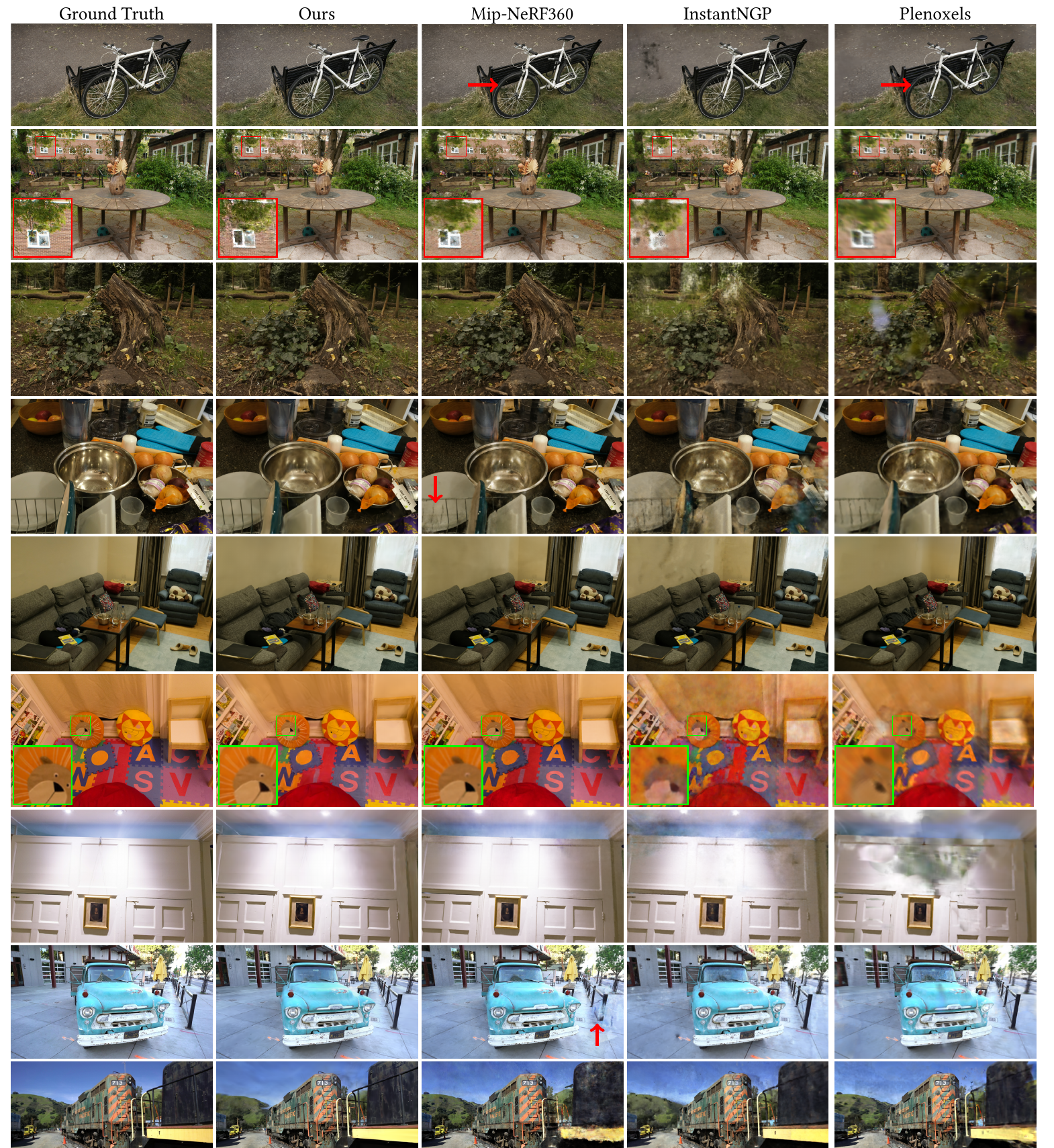
We also show visual results of this comparison for a left-out test view for ours and the previous rendering methods selected for comparison in Figure 5; the results of our method are for 30K iterations of training. We see that in some cases even Mip-NeRF360 has remaining artifacts that our method avoids (e.g., blurriness in vegetation -- in Bicycle, Stump -- or on the walls in Room). In the supplemental video and web page we provide comparisons of paths from a distance. Our method tends to preserve visual detail of well-covered regions even from far away, which is not always the case for previous methods.

图5 还展示了我们的方法和所选既有渲染方法在留出测试视角上的视觉比较；其中我们的方法训练了 30K 次迭代。 可以看到，在某些情况下，即使 Mip-NeRF360 仍存在我们的方法所避免的伪影，例如 Bicycle 和 Stump 中植被的模糊，以及 Room 中墙面的模糊。 补充视频和网页提供了从较远距离观察路径的比较。 即使从远处观察，我们的方法也往往能保留覆盖充分区域的视觉细节，而既有方法并非总能做到。

Synthetic Bounded Scenes. In addition to realistic scenes, we also evaluate our approach on the synthetic Blender dataset. The scenes in question provide an exhaustive set of views, are limited in size, and provide exact camera parameters. In such scenarios, we can achieve state-of-the-art results even with random initialization: we start training from 100K uniformly random Gaussians inside a volume that encloses the scene bounds. Our approach quickly and automatically prunes them to about 6--10K meaningful Gaussians. The final size of the trained model after 30K iterations reaches about 200--500K Gaussians per scene. We report and compare our achieved PSNR scores with previous methods in Table 2 using a white background for compatibility. Examples can be seen in Figure 10 (second image from the left) and in supplemental material. The trained synthetic scenes rendered at 180--300 FPS.

合成有边界场景。 除真实场景外，我们还在合成 Blender 数据集上评估该方法。 这些场景提供完备的视角集合，尺寸有限，并具有精确的相机参数。 在这种场景中，即使随机初始化也能取得先进结果：我们从包围场景边界的体积内均匀随机分布的 100K 个高斯开始训练。 该方法会迅速且自动地将其剪枝为约 6–10K 个有意义的高斯。 训练 30K 次迭代后，每个场景的最终模型约包含 200–500K 个高斯。 为保持兼容性，我们采用白色背景，并在 表2 中报告所达到的 PSNR 分数并与既有方法比较。 示例见 图10 的左起第二张图及补充材料。 训练后的合成场景以 180–300 FPS 渲染。

Compactness. In comparison to previous explicit scene representations, the anisotropic Gaussians used in our optimization are capable of modelling complex shapes with a lower number of parameters. We showcase this by evaluating our approach against the highly compact, point-based models obtained by Zhang et al. We start from their initial point cloud which is obtained by space carving with foreground masks and optimize until we break even with their reported PSNR scores. This usually happens within 2--4 minutes. We surpass their reported metrics using approximately one-fourth of their point count, resulting in an average model size of 3.8 MB, as opposed to their 9 MB. We note that for this experiment, we only used two degrees of our spherical harmonics, similar to theirs.

紧凑性。 与既有显式场景表示相比，优化中使用的各向异性高斯能以更少参数建模复杂形状。 我们通过与 Zhang 等人得到的高度紧凑点模型进行比较来展示这一点。 我们从其使用前景掩码进行空间雕刻所得的初始点云出发，一直优化到与其报告的 PSNR 分数持平。 通常只需 2–4 分钟即可达到这一水平。 我们仅使用其约四分之一的点数便超过其报告指标，平均模型大小为 3.8 MB，而其模型为 9 MB。 需要指出的是，该实验只使用两阶球谐函数，与其设置相似。

7.3 Ablations

We isolated the different contributions and algorithmic choices we made and constructed a set of experiments to measure their effect. Specifically we test the following aspects of our algorithm: initialization from SfM, our densification strategies, anisotropic covariance, the fact that we allow an unlimited number of splats to have gradients and use of spherical harmonics. The quantitative effect of each choice is summarized in Table 3.

我们隔离了不同贡献与算法选择，并构建一组实验衡量其影响。 具体测试内容包括：使用 SfM 初始化、密度化策略、各向异性协方差、允许不限数量的泼溅基元获得梯度，以及使用球谐函数。 各项选择的定量影响汇总于 表3。

图7：使用 SfM 点进行初始化有所帮助。上：使用随机点云初始化；下：使用 SfM 点初始化。

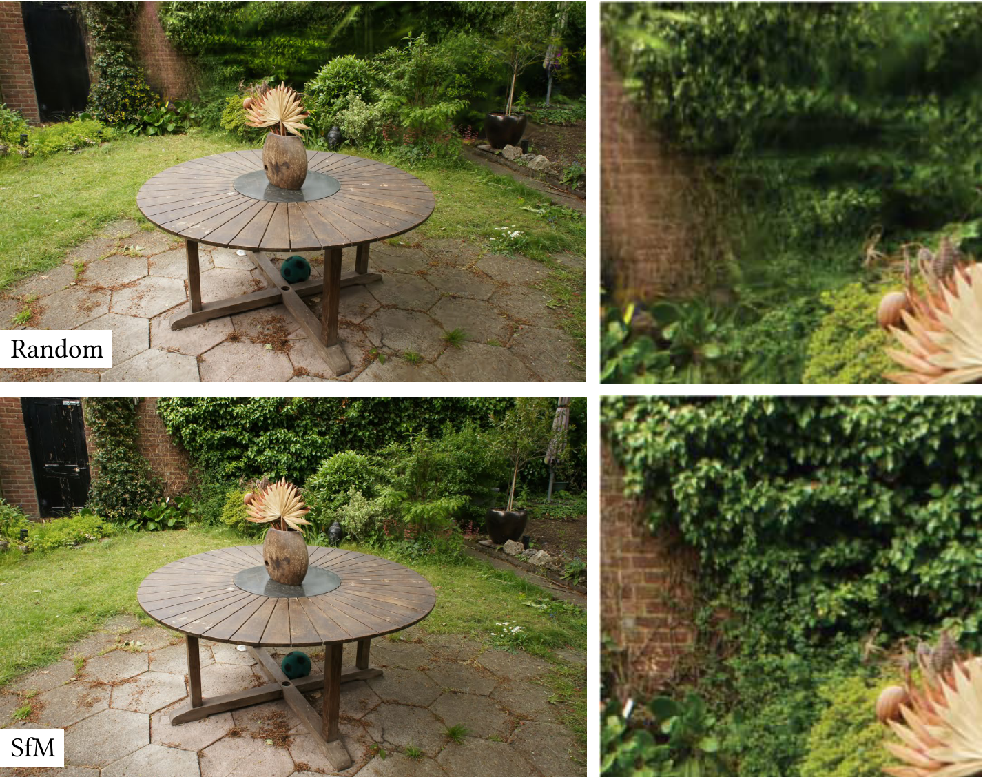
Initialization from SfM. We also assess the importance of initializing the 3D Gaussians from the SfM point cloud. For this ablation, we uniformly sample a cube with a size equal to three times the extent of the input camera's bounding box. We observe that our method performs relatively well, avoiding complete failure even without the SfM points. Instead, it degrades mainly in the background, see Figure 7. Also in areas not well covered from training views, the random initialization method appears to have more floaters that cannot be removed by optimization. On the other hand, the synthetic NeRF dataset does not have this behavior because it has no background and is well constrained by the input cameras (see discussion above).

使用 SfM 初始化。 我们还评估了从 SfM 点云初始化 3D 高斯的重要性。 在该消融实验中，我们在边长为输入相机包围盒范围三倍的立方体内进行均匀采样。 观察发现，即使不使用 SfM 点，该方法仍表现相对良好，并未完全失败。 性能下降主要出现在背景中，见 图7。 在训练视角覆盖不足的区域，随机初始化似乎还会产生更多无法通过优化消除的漂浮伪影。 另一方面，合成 NeRF 数据集没有这种现象，因为它不含背景，且受到输入相机的充分约束，参见前文讨论。

图8：对第 5 节所述“克隆”和“分裂”两种情况的密度化策略进行消融。

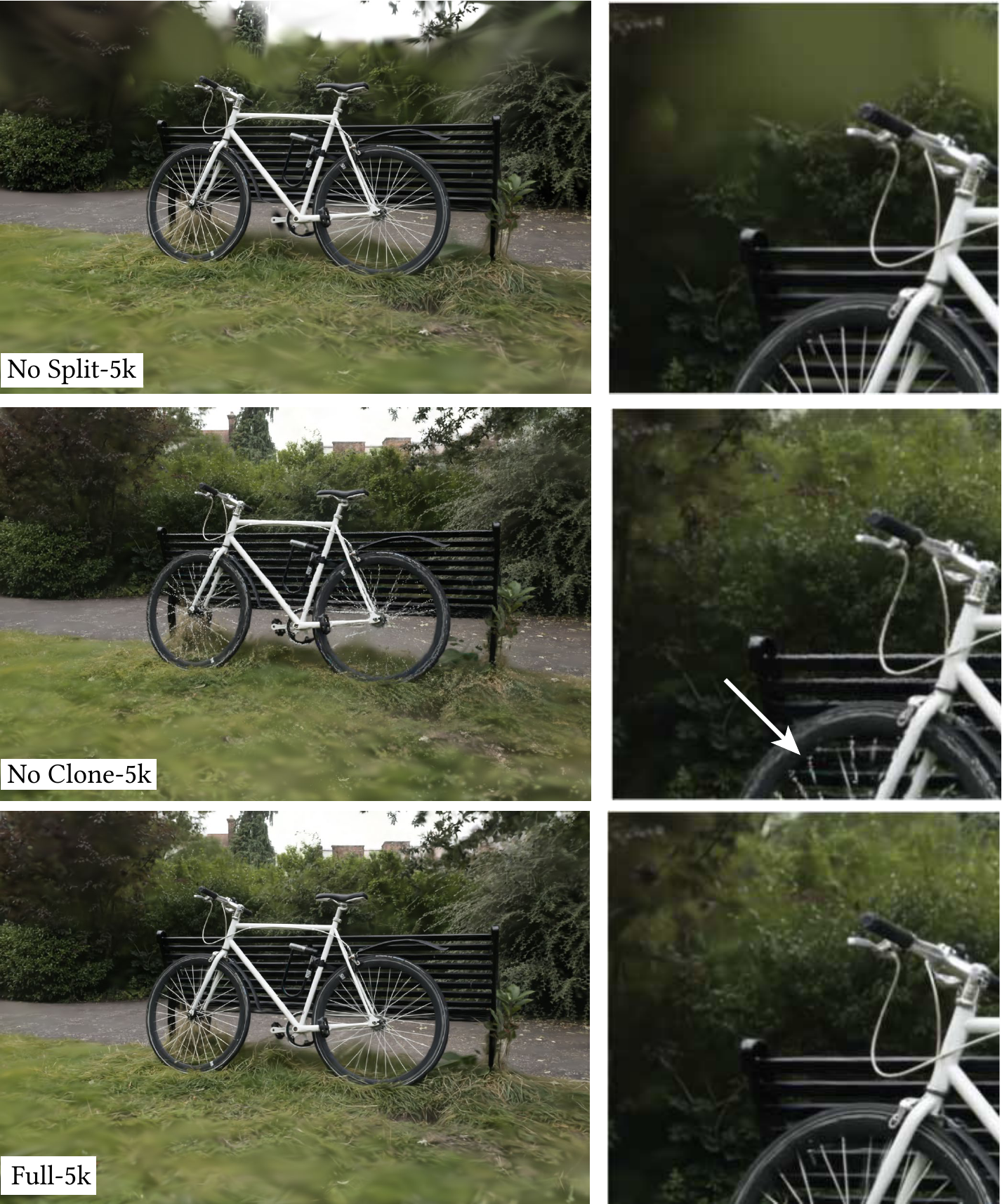
Densification. We next evaluate our two densification methods, more specifically the clone and split strategy described in Section 5. We disable each method separately and optimize using the rest of the method unchanged. Results show that splitting big Gaussians is important to allow good reconstruction of the background as seen in Figure 8, while cloning the small Gaussians instead of splitting them allows for a better and faster convergence especially when thin structures appear in the scene.

密度化。 接下来评估第 5 节所述的两种密度化方法，即克隆与分裂策略。 我们分别禁用其中一种方法，并保持其余部分不变进行优化。 结果表明，如 图8 所示，分裂大型高斯对于良好重建背景十分重要；而克隆小型高斯而非将其分裂，则能实现更好、更快的收敛，尤其是在场景包含细长结构时。

图9：限制获得梯度的点数量会显著影响视觉质量。左：仅允许 10 个高斯获得梯度；右：完整方法。

Unlimited depth complexity of splats with gradients. We evaluate if skipping the gradient computation after the $N$ front-most points will give us speed without sacrificing quality, as suggested in Pulsar. In this test, we choose $N=10$, which is two times higher than the default value in Pulsar, but it led to unstable optimization because of the severe approximation in the gradient computation. For the Truck scene, quality degraded by 11dB in PSNR (see Table 3, Limited-BW), and the visual outcome is shown in Figure 9 for Garden.

获得梯度的泼溅基元具有无限深度复杂度。 我们评估在最靠前的 $N$ 个点之后跳过梯度计算，能否像 Pulsar 所建议的那样，在不牺牲质量的情况下提高速度。 该实验选择 $N=10$，是 Pulsar 默认值的两倍，但梯度计算中的严重近似导致优化不稳定。 在 Truck 场景中，PSNR 下降 11dB，见 表3 的 Limited-BW；Garden 场景的视觉结果见 图9。

Anisotropic Covariance. An important algorithmic choice in our method is the optimization of the full covariance matrix for the 3D Gaussians. To demonstrate the effect of this choice, we perform an ablation where we remove anisotropy by optimizing a single scalar value that controls the radius of the 3D Gaussian on all three axes. The results of this optimization are presented visually in Figure 10. We observe that the anisotropy significantly improves the quality of the 3D Gaussian's ability to align with surfaces, which in turn allows for much higher rendering quality while maintaining the same number of points.

各向异性协方差。 该方法的一项重要算法选择是优化 3D 高斯的完整协方差矩阵。 为展示这一选择的影响，我们进行一项移除各向异性的消融实验，只优化一个控制 3D 高斯在三个轴向上半径的标量。 优化结果在 图10 中进行了可视化展示。 我们观察到，各向异性显著提高了 3D 高斯与表面对齐的能力，因此能够在保持相同点数的同时实现高得多的渲染质量。

图10：分别在禁用和启用高斯各向异性的情况下训练场景。各向异性体积泼溅可以建模细微结构，并显著影响视觉质量。为便于说明，两种配置中的 Ficus 均被限制为最多使用 5K 个高斯。

Spherical Harmonics. Finally, the use of spherical harmonics improves our overall PSNR scores since they compensate for the view-dependent effects (Table 3).

球谐函数。 最后，球谐函数能够补偿视角相关效应，因此提高了整体 PSNR 分数，见 表3。

7.4 Limitations

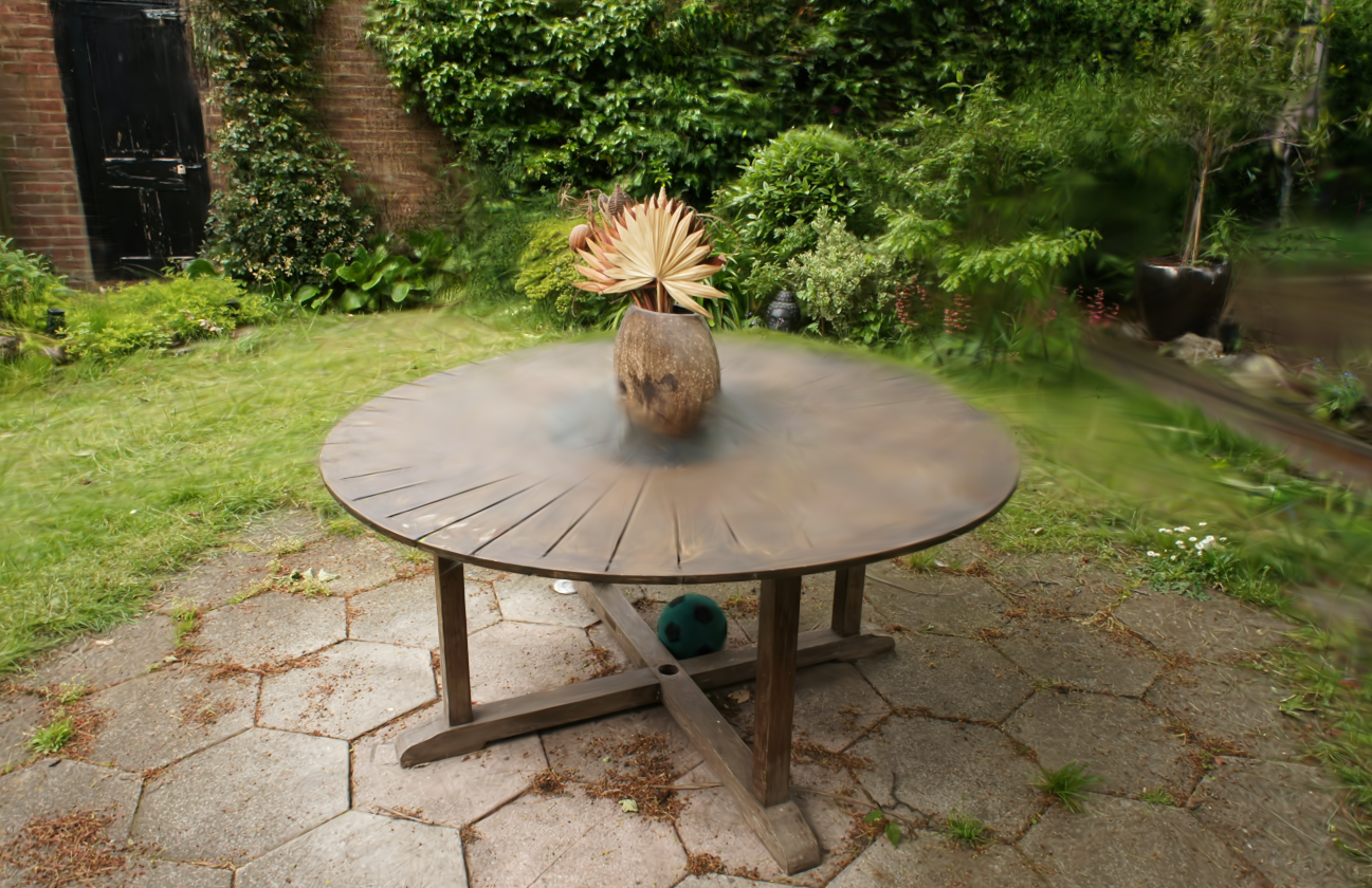
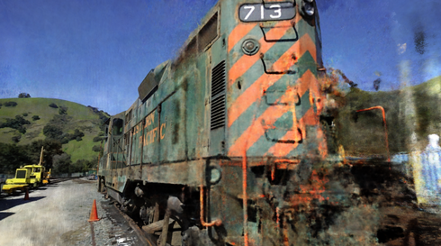
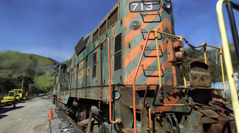
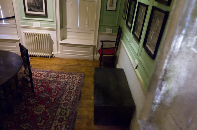
Our method is not without limitations. In regions where the scene is not well observed we have artifacts; in such regions, other methods also struggle (e.g., Mip-NeRF360 in Figure 11). Even though the anisotropic Gaussians have many advantages as described above, our method can create elongated artifacts or "splotchy" Gaussians (see Figure 12); again previous methods also struggle in these cases.

该方法也并非没有局限。 在场景观测不充分的区域会产生伪影，其他方法在这些区域同样面临困难，例如 图11 中的 Mip-NeRF360。 尽管各向异性高斯具有前述诸多优点，该方法仍可能产生细长伪影或“斑块状”高斯，见 图12；既有方法在这些情况下也同样困难。

We also occasionally have popping artifacts when our optimization creates large Gaussians; this tends to happen in regions with view-dependent appearance. One reason for these popping artifacts is the trivial rejection of Gaussians via a guard band in the rasterizer. A more principled culling approach would alleviate these artifacts. Another factor is our simple visibility algorithm, which can lead to Gaussians suddenly switching depth/blending order. This could be addressed by antialiasing, which we leave as future work. Also, we currently do not apply any regularization to our optimization; doing so would help with both the unseen region and popping artifacts.

当优化产生大型高斯时，偶尔还会出现跳变伪影；这种情况往往发生在具有视角相关外观的区域。 产生这类跳变伪影的一个原因，是光栅化器通过保护带直接拒绝高斯。 更合理的剔除方法可以缓解这些伪影。 另一个因素是简单的可见性算法，它可能导致高斯突然切换深度或混合顺序。 抗锯齿可以解决这一问题，我们将其留作未来工作。 此外，目前的优化未采用任何正则化；加入正则化将同时改善未观测区域和跳变伪影。

While we used the same hyperparameters for our full evaluation, early experiments show that reducing the position learning rate can be necessary to converge in very large scenes (e.g., urban datasets).

尽管完整评估统一使用相同超参数，早期实验表明，在非常大的场景中，例如城市场景数据集，可能需要降低位置学习率才能收敛。

Even though we are very compact compared to previous point-based approaches, our memory consumption is significantly higher than NeRF-based solutions. During training of large scenes, peak GPU memory consumption can exceed 20 GB in our unoptimized prototype. However, this figure could be significantly reduced by a careful low-level implementation of the optimization logic (similar to InstantNGP). Rendering the trained scene requires sufficient GPU memory to store the full model (several hundred megabytes for large-scale scenes) and an additional 30--500 MB for the rasterizer, depending on scene size and image resolution. We note that there are many opportunities to further reduce memory consumption of our method. Compression techniques for point clouds is a well-studied field; it would be interesting to see how such approaches could be adapted to our representation.

尽管与既有点渲染方法相比十分紧凑，我们的内存消耗仍显著高于基于 NeRF 的方案。 在大型场景训练期间，未经优化的原型峰值 GPU 内存消耗可能超过 20 GB。 不过，通过谨慎地底层实现优化逻辑，类似 InstantNGP，可以显著降低该数值。 渲染训练后的场景需要足够的 GPU 内存存储完整模型，大规模场景约需数百 MB；此外，光栅化器还需额外 30–500 MB，具体取决于场景大小和图像分辨率。 我们的方法仍有许多进一步降低内存消耗的机会。 点云压缩技术已经得到充分研究，如何将这些方法适配到该表示上值得探索。

图11：失败伪影比较：Mip-NeRF360 存在“漂浮物”和颗粒状外观（左，前景），而我们的方法会产生粗糙的各向异性高斯，导致低细节视觉效果（右，背景）。场景为 Train。

图12：在与训练视角重叠很少的视图中，我们的方法可能产生伪影（右）。Mip-NeRF360 在这些情况下同样会产生伪影（左）。场景为 DrJohnson。

8. Discussion and Conclusions

We have presented the first approach that truly allows real-time, high-quality radiance field rendering, in a wide variety of scenes and capture styles, while requiring training times competitive with the fastest previous methods.

我们提出了首个真正实现实时、高质量辐射场渲染的方法，它适用于多种场景和捕获方式，且训练时间可与此前最快的方法竞争。

Our choice of a 3D Gaussian primitive preserves properties of volumetric rendering for optimization while directly allowing fast splat-based rasterization. Our work demonstrates that -- contrary to widely accepted opinion -- a continuous representation is not strictly necessary to allow fast and high-quality radiance field training.

我们选择 3D 高斯基元，既保留了体积渲染有利于优化的性质，也直接支持快速的泼溅式光栅化。 该工作表明，与广泛接受的观点相反，要实现快速且高质量的辐射场训练，连续表示并非严格必要。

The majority ($\sim$ 80%) of our training time is spent in Python code, since we built our solution in PyTorch to allow our method to be easily used by others. Only the rasterization routine is implemented as optimized CUDA kernels. We expect that porting the remaining optimization entirely to CUDA, as e.g., done in InstantNGP, could enable significant further speedup for applications where performance is essential.

由于方案使用 PyTorch 构建，便于他人使用，训练时间的大部分（$\sim$ 80%）耗费在 Python 代码上。 只有光栅化例程被实现为优化后的 CUDA 核函数。 我们预计，若像 InstantNGP 那样将其余优化过程完全移植到 CUDA，可为性能至关重要的应用带来显著的进一步加速。

We also demonstrated the importance of building on real-time rendering principles, exploiting the power of the GPU and speed of software rasterization pipeline architecture. These design choices are the key to performance both for training and real-time rendering, providing a competitive edge in performance over previous volumetric ray-marching.

我们还展示了以实时渲染原则为基础、利用 GPU 算力和软件光栅化流水线架构速度的重要性。 这些设计选择是训练与实时渲染性能的关键，使其相较既有体积射线步进方法具有性能优势。

It would be interesting to see if our Gaussians can be used to perform mesh reconstructions of the captured scene. Aside from practical implications given the widespread use of meshes, this would allow us to better understand where our method stands exactly in the continuum between volumetric and surface representations.

探索这些高斯能否用于对捕获场景进行网格重建将很有意义。 鉴于网格应用广泛，这不仅具有实践意义，也有助于更准确地理解该方法在体积表示与表面表示连续谱中的位置。

In conclusion, we have presented the first real-time rendering solution for radiance fields, with rendering quality that matches the best expensive previous methods, with training times competitive with the fastest existing solutions.

总之，我们提出了首个辐射场实时渲染方案，其渲染质量可媲美代价高昂的最佳既有方法，而训练时间可与现有最快方案竞争。