---

Visualizing the Loss Landscape of Neural Nets

Li H, Xu Z, Taylor G, Studer C, Goldstein T. Visualizing the Loss Landscape of Neural Nets. NeurIPS 2018.

https://github.com/tomgoldstein/loss-landscape

OptimizationVisualization3190+NeurIPS 2018UMDUSNACornell

---

神经网络损失景观可视化

Abstract

Neural network training relies on our ability to find "good" minimizers of highly non-convex loss functions. It is well-known that certain network architecture designs (e.g., skip connections) produce loss functions that train easier, and well-chosen training parameters (batch size, learning rate, optimizer) produce minimizers that generalize better. However, the reasons for these differences, and their effects on the underlying loss landscape, are not well understood. In this paper, we explore the structure of neural loss functions, and the effect of loss landscapes on generalization, using a range of visualization methods. First, we introduce a simple "filter normalization" method that helps us visualize loss function curvature and make meaningful side-by-side comparisons between loss functions. Then, using a variety of visualizations, we explore how network architecture affects the loss landscape, and how training parameters affect the shape of minimizers.

神经网络训练依赖于我们找到高度非凸损失函数的“好”极小值点的能力。 众所周知，某些网络架构设计（例如 skip connections）会产生更容易训练的损失函数，而选择得当的训练参数（batch size、learning rate、optimizer）会产生泛化更好的极小值点。 然而，这些差异的原因，以及它们对底层损失景观的影响，仍未得到充分理解。 在本文中，作者使用一系列可视化方法，探索神经损失函数的结构，以及损失景观对泛化的影响。 首先，作者引入一种简单的“filter normalization”方法，帮助可视化损失函数曲率，并在损失函数之间进行有意义的并排比较。 然后，作者通过多种可视化，探索网络架构如何影响损失景观，以及训练参数如何影响极小值点的形状。

1. Introduction

Training neural networks requires minimizing a high-dimensional non-convex loss function -- a task that is hard in theory, but sometimes easy in practice. Despite the NP-hardness of training general neural loss functions, simple gradient methods often find global minimizers (parameter configurations with zero or near-zero training loss), even when data and labels are randomized before training. However, this good behavior is not universal; the trainability of neural nets is highly dependent on network architecture design choices, the choice of optimizer, variable initialization, and a variety of other considerations. Unfortunately, the effect of each of these choices on the structure of the underlying loss surface is unclear. Because of the prohibitive cost of loss function evaluations (which requires looping over all the data points in the training set), studies in this field have remained predominantly theoretical.

训练神经网络需要最小化一个高维非凸损失函数，这个任务在理论上很难，但在实践中有时很容易。 尽管训练一般神经损失函数是 NP-hard 的，简单的梯度方法仍经常找到全局极小值点（训练损失为零或接近零的参数配置），即使在训练前把数据和标签随机化也是如此。 然而，这种良好行为并不普遍；神经网络的可训练性高度依赖网络架构设计选择、优化器选择、变量初始化以及其他多种因素。 遗憾的是，这些选择各自对底层损失曲面结构的影响尚不清楚。 由于损失函数评估成本极高（需要遍历训练集中的所有数据点），该领域的研究一直主要停留在理论层面。

图1：The loss surfaces of ResNet-56 with/without skip connections. The proposed filter normalization scheme is used to enable comparisons of sharpness/flatness between the two figures.

Visualizations have the potential to help us answer several important questions about why neural networks work. In particular, why are we able to minimize highly non-convex neural loss functions? And why do the resulting minima generalize? To clarify these questions, we use high-resolution visualizations to provide an empirical characterization of neural loss functions, and explore how different network architecture choices affect the loss landscape. Furthermore, we explore how the non-convex structure of neural loss functions relates to their trainability, and how the geometry of neural minimizers (i.e., their sharpness/flatness, and their surrounding landscape), affects their generalization properties.

可视化有潜力帮助我们回答关于神经网络为什么有效的几个重要问题。 尤其是，为什么我们能够最小化高度非凸的神经损失函数？ 以及，为什么得到的极小值点能够泛化？ 为了澄清这些问题，作者使用高分辨率可视化来对神经损失函数进行经验刻画，并探索不同网络架构选择如何影响损失景观。 此外，作者探索神经损失函数的非凸结构如何关联其可训练性，以及神经极小值点的几何形状（即它们的尖锐/平坦程度以及周围景观）如何影响其泛化性质。

To do this in a meaningful way, we propose a simple "filter normalization" scheme that enables us to do side-by-side comparisons of different minima found during training. We then use visualizations to explore sharpness/flatness of minimizers found by different methods, as well as the effect of network architecture choices (use of skip connections, number of filters, network depth) on the loss landscape. Our goal is to understand how loss function geometry affects generalization in neural nets.

为了以有意义的方式做到这一点，作者提出一种简单的“filter normalization”方案，使我们能够并排比较训练过程中找到的不同极小值点。 随后，作者使用可视化来探索不同方法找到的极小值点的尖锐/平坦程度，以及网络架构选择（是否使用 skip connections、filter 数量、网络深度）对损失景观的影响。 作者的目标是理解损失函数几何如何影响神经网络中的泛化。

1.1 Contributions

We study methods for producing meaningful loss function visualizations. Then, using these visualization methods, we explore how loss landscape geometry affects generalization error and trainability. More specifically, we address the following issues:

• We reveal faults in a number of visualization methods for loss functions, and show that simple visualization strategies fail to accurately capture the local geometry (sharpness or flatness) of loss function minimizers.

• We present a simple visualization method based on "filter normalization." The sharpness of minimizers correlates well with generalization error when this normalization is used, even when making comparisons across disparate network architectures and training methods. This enables side-by-side comparisons of different minimizers.

• We observe that, when networks become sufficiently deep, neural loss landscapes quickly transition from being nearly convex to being highly chaotic. This transition from convex to chaotic behavior coincides with a dramatic drop in generalization error, and ultimately to a lack of trainability.

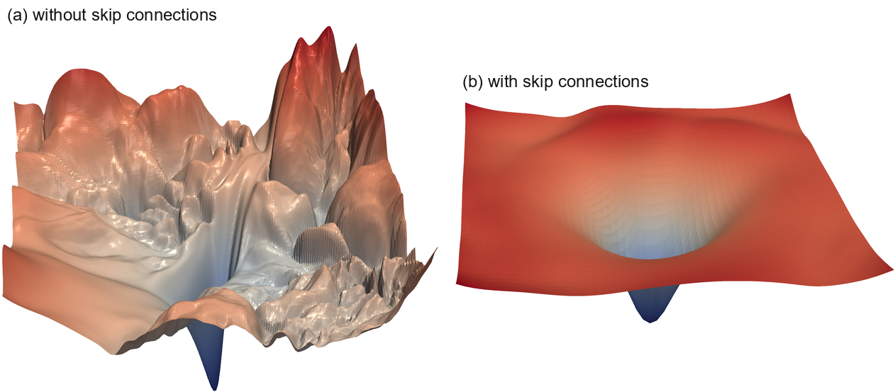
• We observe that skip connections promote flat minimizers and prevent the transition to chaotic behavior, which helps explain why skip connections are necessary for training extremely deep networks.

• We quantitatively measure non-convexity by calculating the smallest (most negative) eigenvalues of the Hessian around local minima, and visualizing the results as a heat map.

• We study the visualization of SGD optimization trajectories. We explain the difficulties that arise when visualizing these trajectories, and show that optimization trajectories lie in an extremely low dimensional space. This low dimensionality can be explained by the presence of large, nearly convex regions in the loss landscape, such as those observed in our 2-dimensional visualizations.

作者研究生成有意义的损失函数可视化的方法。 随后，作者使用这些可视化方法，探索损失景观几何如何影响泛化误差和可训练性。 更具体地说，作者处理以下问题：

• 作者揭示多种损失函数可视化方法中的缺陷，并表明简单的可视化策略无法准确捕捉损失函数极小值点的局部几何（尖锐或平坦）。

• 作者提出一种基于“filter normalization”的简单可视化方法。使用这种归一化时，即使跨不同网络架构和训练方法进行比较，极小值点的尖锐程度也与泛化误差良好相关。这使得不同极小值点之间的并排比较成为可能。

• 作者观察到，当网络变得足够深时，神经损失景观会快速从近似凸转变为高度混沌。这种从凸到混沌的转变伴随着泛化误差的急剧下降，并最终导致不可训练。

• 作者观察到，skip connections 会促进平坦极小值点并阻止向混沌行为的转变，这有助于解释为什么训练极深网络需要 skip connections。

• 作者通过计算局部极小值点附近 Hessian 的最小（最负）特征值，并把结果可视化为热力图，来定量测量非凸性。

• 作者研究 SGD 优化轨迹的可视化。作者解释可视化这些轨迹时出现的困难，并表明优化轨迹位于极低维空间中。这种低维性可以由损失景观中存在大的、近似凸的区域来解释，例如作者在二维可视化中观察到的那些区域。

2. Theoretical Background

Numerous theoretical studies have been done on our ability to optimize neural loss function. Theoretical results usually make restrictive assumptions about the sample distributions, non-linearity of the architecture, or loss functions. For restricted network classes, such as those with a single hidden layer, globally optimal or near-optimal solutions can be found by common optimization methods. For networks with specific structures, there likely exists a monotonically decreasing path from an initialization to a global minimum. Swirszcz et al. show counterexamples that achieve "bad" local minima for toy problems.

关于我们优化神经损失函数的能力，已经有大量理论研究。 理论结果通常会对样本分布、架构的非线性或损失函数作出限制性假设。 对于受限的网络类别，例如只有单个隐藏层的网络，常见优化方法可以找到全局最优或近似最优解。 对于具有特定结构的网络，很可能存在一条从初始化到全局极小值单调下降的路径。 Swirszcz 等人给出了一些反例，这些反例在玩具问题上达到“坏”的局部极小值。

Several works have addressed the relationship between sharpness/flatness of local minima and their generalization ability. Hochreiter and Schmidhuber defined "flatness" as the size of the connected region around the minimum where the training loss remains low. Keskar et al. characterize flatness using eigenvalues of the Hessian, and propose $ϵ$-sharpness as an approximation, which looks at the maximum loss in a neighborhood of a minimum. Dinh et al. and Neyshabur et al. show that these quantitative measure of sharpness are not invariant to symmetries in the network, and are thus not sufficient to determine generalization ability. Entropy-SGD used local entropy as a measure of sharpness, which is invariant to the simple transformation in Dinh et al., but difficult to accurately compute. Dziugaite and Roy connect sharpness to PAC-Bayes bounds for generalization.

已有若干工作讨论了局部极小值的尖锐/平坦程度与其泛化能力之间的关系。 Hochreiter 和 Schmidhuber 将“flatness”定义为极小值周围训练损失保持较低的连通区域大小。 Keskar 等人使用 Hessian 的特征值来刻画平坦性，并提出 $ϵ$-sharpness 作为近似，该近似考察极小值邻域中的最大损失。 Dinh 等人和 Neyshabur 等人表明，这些尖锐程度的定量度量对网络中的对称性并不不变，因此不足以决定泛化能力。 Entropy-SGD 使用局部熵作为尖锐程度的度量，它对 Dinh 等人中的简单变换是不变的，但难以准确计算。 Dziugaite 和 Roy 将尖锐程度与泛化的 PAC-Bayes 界联系起来。

3. The Basics of Loss Function Visualization

Neural networks are trained on a corpus of feature vectors (e.g., images) $\{x_i\}$ and accompanying labels $\{y_i\}$ by minimizing a loss of the form

$$L(\theta )=\frac{1}{m}\sum _{i=1}^m\ell (x_i,y_i;\theta ),$$

where $\theta$ denotes the parameters (weights) of the neural network, the function $\ell (x_i,y_i;\theta )$ measures how well the neural network with parameters $\theta$ predicts the label of a data sample, and $m$ is the number of data samples. Neural nets contain many parameters, and so their loss functions live in a very high-dimensional space. Unfortunately, visualizations are only possible using low-dimensional 1D (line) or 2D (surface) plots. Several methods exist for closing this dimensionality gap.

神经网络通过最小化如下形式的损失，在一组特征向量（例如图像）$\{x_i\}$ 及其对应标签 $\{y_i\}$ 上训练：

$$L(\theta )=\frac{1}{m}\sum _{i=1}^m\ell (x_i,y_i;\theta ),$$

其中 $\theta$ 表示神经网络的参数（权重），函数 $\ell (x_i,y_i;\theta )$ 衡量参数为 $\theta$ 的神经网络预测某个数据样本标签的效果，$m$ 是数据样本数量。 神经网络包含许多参数，因此它们的损失函数存在于非常高维的空间中。 遗憾的是，可视化只能使用低维的一维（线）或二维（曲面）图。 已有若干方法用于弥合这种维度差距。

1-Dimensional Linear Interpolation. One simple and lightweight way to plot loss functions is to choose two sets of parameters $\theta$ and ${\theta }^{\prime },$ and plot the values of the loss function along the line connecting these two points. We can parameterize this line by choosing a scalar parameter $\alpha ,$ and defining the weighted average

$$\theta (\alpha )=(1-\alpha )\theta +\alpha {\theta }^{\prime }.$$

Finally, we plot the function $f(\alpha )=L(\theta (\alpha )).$ This strategy was taken by Goodfellow et al., who studied the loss surface along the line between a random initial guess, and a nearby minimizer obtained by stochastic gradient descent. This method has been widely used to study the "sharpness" and "flatness" of different minima, and the dependence of sharpness on batch-size. Smith and Topin use the same technique to show different minima and the "peaks" between them, while Im et al. plot the line between minima obtained via different optimizers.

一维线性插值。 绘制损失函数的一种简单且轻量的方法，是选择两组参数 $\theta$ 和 ${\theta }^{\prime }$，并沿连接这两个点的直线绘制损失函数值。 我们可以通过选择标量参数 $\alpha$ 来参数化这条直线，并定义加权平均：

$$\theta (\alpha )=(1-\alpha )\theta +\alpha {\theta }^{\prime }.$$

最后，我们绘制函数 $f(\alpha )=L(\theta (\alpha ))$。 Goodfellow 等人采用了这一策略，他们研究了随机初始猜测与随机梯度下降得到的附近极小值点之间直线上的损失曲面。 这种方法已被广泛用于研究不同极小值的“sharpness”和“flatness”，以及尖锐程度对 batch-size 的依赖。 Smith 和 Topin 使用同一技术展示不同极小值及其之间的“peaks”，而 Im 等人绘制了由不同优化器获得的极小值之间的直线。

The 1D linear interpolation method suffers from several weaknesses. First, it is difficult to visualize non-convexities using 1D plots. Indeed, Goodfellow et al. found that loss functions appear to lack local minima along the minimization trajectory. We will see later, using 2D methods, that some loss functions have extreme non-convexities, and that these non-convexities correlate with the difference in generalization between different network architectures. Second, this method does not consider batch normalization or invariance symmetries in the network. For this reason, the visual sharpness comparisons produced by 1D interpolation plots may be misleading; this issue will be explored in depth in Section 5.

一维线性插值方法存在若干弱点。 首先，使用一维图很难可视化非凸性。 实际上，Goodfellow 等人发现，沿最小化轨迹观察时，损失函数似乎缺少局部极小值。 后文会看到，使用二维方法时，一些损失函数具有极端的非凸性，而且这些非凸性与不同网络架构之间的泛化差异相关。 其次，这种方法没有考虑 batch normalization 或网络中的不变对称性。 因此，一维插值图产生的视觉尖锐程度比较可能具有误导性；这一问题将在第 5 节中深入探讨。

Contour Plots & Random Directions. To use this approach, one chooses a center point ${\theta }^{\ast }$ in the graph, and chooses two direction vectors, $\delta$ and $\eta$. One then plots a function of the form $f(\alpha )=L({\theta }^{\ast }+\alpha \delta )$ in the 1D (line) case, or

$$f(\alpha ,\beta )=L({\theta }^{\ast }+\alpha \delta +\beta \eta )$$

in the 2D (surface) case. When making 2D plots in this paper, batch normalization parameters are held constant, i.e., random directions are not applied to batch normalization parameters. This approach was used by Goodfellow et al. to explore the trajectories of different minimization methods. It was also used by Im et al. to show that different optimization algorithms find different local minima within the 2D projected space. Because of the computational burden of 2D plotting, these methods generally result in low-resolution plots of small regions that have not captured the complex non-convexity of loss surfaces. Below, we use high-resolution visualizations over large slices of weight space to visualize how network design affects non-convex structure.

等高线图与随机方向。 要使用这种方法，需要在图中选择一个中心点 ${\theta }^{\ast }$，并选择两个方向向量 $\delta$ 和 $\eta$。 随后，在一维（线）情况下绘制形如 $f(\alpha )=L({\theta }^{\ast }+\alpha \delta )$ 的函数，或者在二维（曲面）情况下绘制：

$$f(\alpha ,\beta )=L({\theta }^{\ast }+\alpha \delta +\beta \eta ).$$

在二维（曲面）情况下使用上述形式。 本文制作二维图时，batch normalization 参数保持不变，即随机方向不会作用于 batch normalization 参数。 Goodfellow 等人曾使用这种方法来探索不同最小化方法的轨迹。 Im 等人也使用该方法表明，不同优化算法会在二维投影空间中找到不同的局部极小值。 由于二维绘图计算负担很重，这些方法通常只能得到小区域的低分辨率图，无法捕捉损失曲面的复杂非凸性。 下文中，作者在权重空间的大切片上使用高分辨率可视化，来展示网络设计如何影响非凸结构。

4. Proposed Visualization: Filter-Wise Normalization

This study relies heavily on plots of the form $f(\alpha ,\beta )=L({\theta }^{\ast }+\alpha \delta +\beta \eta )$ produced using random direction vectors, $\delta$ and $\eta ,$ each sampled from a random Gaussian distribution with appropriate scaling (described below). While the "random directions" approach to plotting is simple, it fails to capture the intrinsic geometry of loss surfaces, and cannot be used to compare the geometry of two different minimizers or two different networks. This is because of the scale invariance in network weights. When ReLU non-linearities are used, the network remains unchanged if we (for example) multiply the weights in one layer of a network by 10, and divide the next layer by 10. This invariance is even more prominent when batch normalization is used. In this case, the size (i.e., norm) of a filter is irrelevant because the output of each layer is re-scaled during batch normalization. For this reason, a network's behavior remains unchanged if we re-scale the weights. Note, this scale invariance applies only to rectified networks.

本研究高度依赖形如 $f(\alpha ,\beta )=L({\theta }^{\ast }+\alpha \delta +\beta \eta )$ 的图，这些图使用随机方向向量 $\delta$ 和 $\eta$ 生成，每个方向都从随机高斯分布中采样并采用适当缩放（如下所述）。 虽然“random directions”绘图方法很简单，但它无法捕捉损失曲面的内在几何，也不能用于比较两个不同极小值点或两个不同网络的几何。 这是因为网络权重存在尺度不变性。 当使用 ReLU 非线性时，如果我们（例如）将网络某一层的权重乘以 10，并将下一层除以 10，网络保持不变。 使用 batch normalization 时，这种不变性更加明显。 在这种情况下，filter 的大小（即范数）无关紧要，因为每一层的输出会在 batch normalization 过程中被重新缩放。 因此，如果我们重新缩放权重，网络行为保持不变。 需要注意的是，这种尺度不变性只适用于整流网络。

Scale invariance prevents us from making meaningful comparisons between plots, unless special precautions are taken. A neural network with large weights may appear to have a smooth and slowly varying loss function; perturbing the weights by one unit will have very little effect on network performance if the weights live on a scale much larger than one. However, if the weights are much smaller than one, then that same unit perturbation may have a catastrophic effect, making the loss function appear quite sensitive to weight perturbations. Keep in mind that neural nets are scale invariant; if the small-parameter and large-parameter networks in this example are equivalent (because one is simply a rescaling of the other), then any apparent differences in the loss function are merely an artifact of scale invariance. This scale invariance was exploited by Dinh et al. to build pairs of equivalent networks that have different apparent sharpness.

除非采取特殊预防措施，否则尺度不变性会阻碍我们在图之间进行有意义的比较。 一个权重很大的神经网络可能看起来具有平滑且缓慢变化的损失函数；如果权重所处尺度远大于 1，那么对权重施加一个单位的扰动对网络性能影响很小。 然而，如果权重远小于 1，同样的单位扰动可能产生灾难性影响，使损失函数看起来对权重扰动非常敏感。 请记住，神经网络具有尺度不变性；如果这个例子中的小参数网络和大参数网络是等价的（因为一个只是另一个的重新缩放），那么损失函数中的任何表面差异都只是尺度不变性的伪影。 Dinh 等人利用这种尺度不变性构造了成对的等价网络，但它们具有不同的表观尖锐程度。

To remove this scaling effect, we plot loss functions using filter-wise normalized directions. To obtain such directions for a network with parameters $\theta ,$ we begin by producing a random Gaussian direction vector $d$ with dimensions compatible with $\theta$. Then, we normalize each filter in $d$ to have the same norm of the corresponding filter in $\theta .$ In other words, we make the replacement

$$d_{i,j}\leftarrow \frac{d_{i,j}}{\parallel d_{i,j}\parallel }\parallel {\theta }_{i,j}\parallel ,$$

where $d_{i,j}$ represents the $j$th filter (not the $j$th weight) of the $i$th layer of $d$, and $\parallel \cdot \parallel$ denotes the Frobenius norm. Note that the filter-wise normalization is different from that of Im et al., which normalize the direction without considering the norm of individual filters. Note that filter normalization is not limited to convolutional (Conv) layers but also applies to fully connected (FC) layers. The FC layer is equivalent to a Conv layer with a $1\times 1$ output feature map and the filter corresponds to the weights that generate one neuron.

为了移除这种缩放效应，作者使用 filter-wise normalized directions 来绘制损失函数。 为了为参数为 $\theta$ 的网络获得这样的方向，作者首先生成一个与 $\theta$ 维度兼容的随机高斯方向向量 $d$。 然后，作者将 $d$ 中的每个 filter 归一化，使其与 $\theta$ 中对应 filter 具有相同范数。 换言之，作者进行如下替换：

$$d_{i,j}\leftarrow \frac{d_{i,j}}{\parallel d_{i,j}\parallel }\parallel {\theta }_{i,j}\parallel .$$

其中 $d_{i,j}$ 表示 $d$ 的第 $i$ 层中的第 $j$ 个 filter（不是第 $j$ 个权重），$\parallel \cdot \parallel$ 表示 Frobenius 范数。 需要注意的是，filter-wise normalization 不同于 Im 等人的方法，后者在不考虑单个 filter 范数的情况下归一化方向。 还要注意，filter normalization 不限于卷积（Conv）层，也适用于全连接（FC）层。 FC 层等价于具有 $1\times 1$ 输出特征图的 Conv 层，而 filter 对应于生成一个神经元的权重。

Do contour plots of the form $f(\alpha ,\beta )=L({\theta }^{\ast }+\alpha \delta +\beta \eta )$ capture the natural distance scale of loss surfaces when the directions $\delta$ and $\eta$ are filter normalized? We answer this question to the affirmative in Section 5 by showing that the sharpness of filter-normalized plots correlates well with generalization error, while plots without filter normalization can be very misleading. In the appendix, we also compare filter-wise normalization to layer-wise normalization (and no normalization), and show that filter normalization produces superior correlation between sharpness and generalization error.

当方向 $\delta$ 和 $\eta$ 经过 filter normalization 时，形如 $f(\alpha ,\beta )=L({\theta }^{\ast }+\alpha \delta +\beta \eta )$ 的等高线图是否捕捉了损失曲面的自然距离尺度？ 作者在第 5 节中肯定回答了这个问题：filter-normalized 图的尖锐程度与泛化误差良好相关，而没有 filter normalization 的图可能非常具有误导性。 在附录中，作者还比较了 filter-wise normalization、layer-wise normalization（以及不做 normalization），并表明 filter normalization 在尖锐程度与泛化误差之间产生更好的相关性。

5. The Sharp vs Flat Dilemma

Section 4 introduces the concept of filter normalization, and provides an intuitive justification for its use. In this section, we address the issue of whether sharp minimizers generalize better than flat minimizers. In doing so, we will see that the sharpness of minimizers correlates well with generalization error when filter normalization is used. This enables side-by-side comparisons between plots. In contrast, the sharpness of non-normalized plots may appear distorted and unpredictable.

第 4 节引入了 filter normalization 的概念，并为其使用提供了直观理由。 在本节中，作者讨论尖锐极小值点是否比平坦极小值点泛化更好的问题。 在此过程中，我们将看到，使用 filter normalization 时，极小值点的尖锐程度与泛化误差良好相关。 这使图之间的并排比较成为可能。 相比之下，未归一化图中的尖锐程度可能显得扭曲且不可预测。

It is widely thought that small-batch SGD produces "flat" minimizers that generalize well, while large batches produce "sharp" minima with poor generalization. This claim is disputed though, with Dinh et al. and Kawaguchi et al. arguing that generalization is not directly related to the curvature of loss surfaces, and some authors proposing specialized training methods that achieve good performance with large batch sizes. Here, we explore the difference between sharp and flat minimizers. We begin by discussing difficulties that arise when performing such a visualization, and how proper normalization can prevent such plots from producing distorted results.

人们普遍认为，small-batch SGD 会产生泛化良好的“flat”极小值点，而 large batches 会产生泛化较差的“sharp”极小值。 不过，这一说法存在争议：Dinh 等人和 Kawaguchi 等人认为泛化并不直接关联损失曲面的曲率，也有一些作者提出了使用 large batch sizes 仍能获得良好性能的专门训练方法。 在这里，作者探索尖锐极小值点和平坦极小值点之间的差异。 作者首先讨论进行这种可视化时出现的困难，以及适当的 normalization 如何防止这类图产生扭曲结果。

We train a CIFAR-10 classifier using a 9-layer VGG network with batch normalization for a fixed number of epochs. We use two batch sizes: a large batch size of 8192 (16.4% of the training data of CIFAR-10), and a small batch size of 128. Let ${\theta }^s$ and ${\theta }^l$ indicate the solutions obtained by running SGD using small and large batch sizes, respectively. In this section, we consider the "running mean" and "running variance" as trainable parameters and include them in $\theta$. Note that the original study by Goodfellow et al. does not consider batch normalization. These parameters are not included in $\theta$ in future sections, as they are only needed when interpolating between two minimizers. Using the linear interpolation approach, we plot the loss values on both training and testing data sets of CIFAR-10, along a direction containing the two solutions, i.e., $f(\alpha )=L({\theta }^s+\alpha ({\theta }^l-{\theta }^s))$.

作者使用带 batch normalization 的 9 层 VGG 网络，在固定 epoch 数下训练 CIFAR-10 分类器。 作者使用两个 batch size：8192 的 large batch size（CIFAR-10 训练数据的 16.4%）和 128 的 small batch size。 令 ${\theta }^s$ 和 ${\theta }^l$ 分别表示使用 small 和 large batch size 运行 SGD 得到的解。 在本节中，作者将“running mean”和“running variance”视为可训练参数，并把它们纳入 $\theta$。 注意，Goodfellow 等人的原始研究没有考虑 batch normalization。 这些参数在后续章节不会纳入 $\theta$，因为它们只在两个极小值点之间插值时需要。 使用线性插值方法，作者沿包含这两个解的方向，在 CIFAR-10 的训练集和测试集上绘制损失值，即 $f(\alpha )=L({\theta }^s+\alpha ({\theta }^l-{\theta }^s))$。

图2：(a) and (d) are the 1D linear interpolation of VGG-9 solutions obtained by small-batch and large-batch training methods. The blue lines are loss values and the red lines are accuracies. The solid lines are training curves and the dashed lines are for testing. Small batch is at abscissa 0, and large batch is at abscissa 1. The corresponding test errors are shown below. (b) and (e) shows the change of weights norm $\parallel \theta {\parallel }_2$ during training. When weight decay is disabled, the weight norm grows steadily during training without constraints. (c) and (f) are the weight histograms, which verify that small-batch methods produce more large weights with zero weight decay and more small weights with non-zero weight decay.

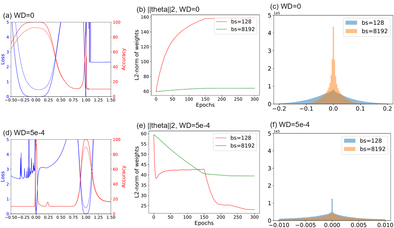
Figure Figure 2(a) shows linear interpolation plots with ${\theta }^s$ at $x$-axis location 0, and ${\theta }^l$ at location 1. As observed by Keskar et al., we can clearly see that the small-batch solution is quite wide, while the large-batch solution is sharp. However, this sharpness balance can be flipped simply by turning on weight decay. Figure Figure 2(d) show results of the same experiment, except this time with a non-zero weight decay parameter. This time, the large batch minimizer is considerably flatter than the sharp small batch minimizer. However, we see that small batches generalize better in all experiments; there is no apparent correlation between sharpness and generalization. We will see that these sharpness comparisons are extremely misleading, and fail to capture the endogenous properties of the minima.

图2(a) 展示了线性插值图，其中 ${\theta }^s$ 位于 $x$ 轴位置 0，${\theta }^l$ 位于位置 1。 正如 Keskar 等人所观察到的，我们可以清楚地看到 small-batch 解相当宽，而 large-batch 解很尖锐。 然而，仅仅打开 weight decay 就可以反转这种尖锐程度的平衡。 图2(d) 展示了同一实验的结果，只是这次使用了非零的 weight decay 参数。 这一次，large batch 极小值点比尖锐的 small batch 极小值点平坦得多。 然而，我们看到 small batches 在所有实验中泛化都更好；尖锐程度和泛化之间没有明显相关性。 我们将看到，这些尖锐程度比较极具误导性，并且未能捕捉极小值点的内生性质。

The apparent differences in sharpness can be explained by examining the weights of each minimizer. Histograms of the network weights are shown for each experiment in Figure Figure 2(c) and (f). We see that, when a large batch is used with zero weight decay, the resulting weights tend to be smaller than in the small batch case. We reverse this effect by adding weight decay; in this case the large batch minimizer has much larger weights than the small batch minimizer. This difference in scale occurs for a simple reason: A smaller batch size results in more weight updates per epoch than a large batch size, and so the shrinking effect of weight decay (which imposes a penalty on the norm of the weights) is more pronounced. The evolution of the weight norms during training is depicted in Figure Figure 2(b) and (e). Figure Figure 2 is not visualizing the endogenous sharpness of minimizers, but rather just the (irrelevant) weight scaling. The scaling of weights in these networks is irrelevant because batch normalization re-scales the outputs to have unit variance. However, small weights still appear more sensitive to perturbations, and produce sharper looking minimizers.

表观尖锐程度的差异可以通过检查每个极小值点的权重来解释。 图2(c) 和 (f) 展示了每个实验中的网络权重直方图。 可以看到，当使用 large batch 且 weight decay 为零时，得到的权重往往比 small batch 情况更小。 加入 weight decay 后，作者反转了这一效应；在这种情况下，large batch 极小值点的权重远大于 small batch 极小值点。 这种尺度差异出现的原因很简单： 较小的 batch size 每个 epoch 会产生比 large batch size 更多的权重更新，因此 weight decay 的收缩效应（它对权重范数施加惩罚）更加明显。 训练过程中权重范数的演化如 图2(b) 和 (e) 所示。 图2 可视化的不是极小值点的内生尖锐程度，而只是（无关的）权重缩放。 这些网络中的权重缩放是无关的，因为 batch normalization 会把输出重新缩放为单位方差。 然而，小权重看起来仍然对扰动更敏感，并产生外观看起来更尖锐的极小值点。

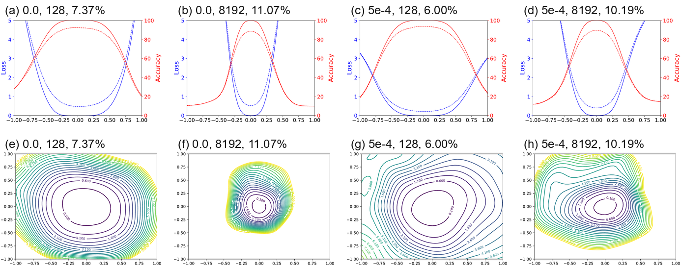
Filter Normalized Plots. We repeat the experiment in Figure Figure 2, but this time we plot the loss function near each minimizer separately using random filter-normalized directions. This removes the apparent differences in geometry caused by the scaling depicted in Figure Figure 2(c) and (f). The results, presented in Figure Figure 3, still show differences in sharpness between small batch and large batch minima, however these differences are much more subtle than it would appear in the un-normalized plots. For comparison, sample un-normalized plots and layer-normalized plots are shown in the appendix. We also visualize these results using two random directions and contour plots. The weights obtained with small batch size and non-zero weight decay have wider contours than the sharper large batch minimizers. Results for ResNet-56 appear in the appendix. Using the filter-normalized plots in Figure Figure 3, we can make side-by-side comparisons between minimizers, and we see that now sharpness correlates well with generalization error. Large batches produced visually sharper minima (although not dramatically so) with higher test error.

Filter Normalized Plots. 作者重复 图2 中的实验，但这次使用随机 filter-normalized directions 分别绘制每个极小值点附近的损失函数。 这移除了 图2(c) 和 (f) 中所示缩放造成的几何表观差异。 图3 展示的结果仍然显示 small batch 和 large batch 极小值之间存在尖锐程度差异，但这些差异比未归一化图中看起来要微妙得多。 作为比较，未归一化图和 layer-normalized 图的示例见附录。 作者还使用两个随机方向和等高线图来可视化这些结果。 使用 small batch size 和非零 weight decay 得到的权重，比更尖锐的 large batch 极小值点具有更宽的等高线。 ResNet-56 的结果见附录。 使用 图3 中的 filter-normalized 图，我们可以并排比较极小值点，并看到尖锐程度现在与泛化误差良好相关。 Large batches 产生了视觉上更尖锐的极小值（尽管并不夸张），并具有更高的测试误差。

图3：The 1D and 2D visualization of solutions obtained using SGD with different weight decay and batch size. The title of each subfigure contains the weight decay, batch size, and test error.

6. What Makes Neural Networks Trainable? Insights on the (Non)Convexity Structure of Loss Surfaces

Our ability to find global minimizers to neural loss functions is not universal; it seems that some neural architectures are easier to minimize than others. For example, using skip connections, the authors of ResNet trained extremely deep architectures, while comparable architectures without skip connections are not trainable. Furthermore, our ability to train seems to depend strongly on the initial parameters from which training starts. Using visualization methods, we do an empirical study of neural architectures to explore why the non-convexity of loss functions seems to be problematic in some situations, but not in others. We aim to provide insight into the following questions: Do loss functions have significant non-convexity at all? If prominent non-convexities exist, why are they not problematic in all situations? Why are some architectures easy to train, and why are results so sensitive to the initialization? We will see that different architectures have extreme differences in non-convexity structure that answer these questions, and that these differences correlate with generalization error.

我们找到神经损失函数全局极小值点的能力并不普遍；一些神经架构似乎比另一些更容易最小化。 例如，ResNet 的作者使用 skip connections 训练了极深架构，而没有 skip connections 的可比架构无法训练。 此外，训练能力似乎强烈依赖训练开始时的初始参数。 作者使用可视化方法，对神经架构进行经验研究，以探索为什么损失函数的非凸性在某些情况下似乎有问题，而在另一些情况下却没有问题。 作者旨在为以下问题提供见解： 损失函数是否真的具有显著非凸性？ 如果存在突出的非凸性，为什么它们并非在所有情况下都有问题？ 为什么某些架构容易训练，为什么结果对初始化如此敏感？ 我们将看到，不同架构在非凸结构上存在极端差异，这些差异回答了这些问题，并且与泛化误差相关。

图4：The loss surfaces of ResNet-110-noshort and DenseNet for CIFAR-10.

Experimental Setup. To understand the effects of network architecture on non-convexity, we trained a number of networks, and plotted the landscape around the obtained minimizers using the filter-normalized random direction method described in Section 4. We consider three classes of neural networks: 1) ResNets that are optimized for performance on CIFAR-10. We consider ResNet-20/56/110, where each name is labeled with the number of layers it has. 2) "VGG-like" networks that do not contain shortcut/skip connections. We produced these networks simply by removing the shortcut connections from ResNets. We call these networks ResNet-20/56/110-noshort. 3) "Wide" ResNets that have more filters per layer than the CIFAR-10 optimized networks. All models are trained on the CIFAR-10 dataset using SGD with Nesterov momentum, batch-size 128, and 0.0005 weight decay for 300 epochs. The learning rate was initialized at 0.1, and decreased by a factor of 10 at epochs 150, 225 and 275. Deeper experimental VGG-like networks (e.g., ResNet-56-noshort, as described below) required a smaller initial learning rate of $0.01$. High resolution 2D plots of the minimizers for different neural networks are shown in Figure Figure 5 and Figure Figure 6. Results are shown as contour plots rather than surface plots because this makes it extremely easy to see non-convex structures and evaluate sharpness. For surface plots of ResNet-56, see Figure Figure 1. Note that the center of each plot corresponds to the minimizer, and the two axes parameterize two random directions with filter-wise normalization as in $f(\alpha ,\beta )=L({\theta }^{\ast }+\alpha \delta +\beta \eta )$. We make several observations below about how architecture affects the loss landscape.

实验设置。 为理解网络架构对非凸性的影响，作者训练了多个网络，并使用第 4 节所述的 filter-normalized random direction 方法，绘制所得极小值点周围的景观。 作者考虑三类神经网络： 1）针对 CIFAR-10 性能优化的 ResNets。 作者考虑 ResNet-20/56/110，其中每个名称都标注了其层数。 2）不包含 shortcut/skip connections 的“VGG-like”网络。 作者通过简单地从 ResNets 中移除 shortcut connections 来产生这些网络。 作者称这些网络为 ResNet-20/56/110-noshort。 3）每层 filter 数量多于 CIFAR-10 优化网络的“Wide”ResNets。 所有模型都在 CIFAR-10 数据集上训练，使用带 Nesterov momentum 的 SGD、batch-size 128 和 0.0005 weight decay，训练 300 个 epochs。 学习率初始化为 0.1，并在第 150、225 和 275 个 epoch 降低 10 倍。 更深的实验性 VGG-like 网络（例如下文所述的 ResNet-56-noshort）需要较小的初始学习率 $0.01$。 不同神经网络极小值点的高分辨率二维图如 图5 和 图6 所示。 结果显示为等高线图而不是曲面图，因为这样可以非常容易地看到非凸结构并评估尖锐程度。 关于 ResNet-56 的曲面图，见 图1。 注意，每个图的中心对应极小值点，两条坐标轴按 $f(\alpha ,\beta )=L({\theta }^{\ast }+\alpha \delta +\beta \eta )$ 中的 filter-wise normalization 参数化两个随机方向。 下面，作者对架构如何影响损失景观作出若干观察。

图5：2D visualization of the loss surface of ResNet and ResNet-noshort with different depth.

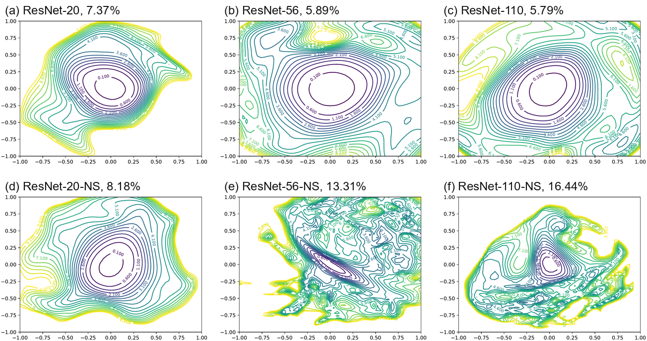
The Effect of Network Depth. From Figure Figure 5, we see that network depth has a dramatic effect on the loss surfaces of neural networks when skip connections are not used. The network ResNet-20-noshort has a fairly benign landscape dominated by a region with convex contours in the center, and no dramatic non-convexity. This isn't too surprising: the original VGG networks for ImageNet had 19 layers and could be trained effectively. However, as network depth increases, the loss surface of the VGG-like nets spontaneously transitions from (nearly) convex to chaotic. ResNet-56-noshort has dramatic non-convexities and large regions where the gradient directions (which are normal to the contours depicted in the plots) do not point towards the minimizer at the center. Also, the loss function becomes extremely large as we move in some directions. ResNet-110-noshort displays even more dramatic non-convexities, and becomes extremely steep as we move in all directions shown in the plot. Furthermore, note that the minimizers at the center of the deep VGG-like nets seem to be fairly sharp. In the case of ResNet-56-noshort, the minimizer is also fairly ill-conditioned, as the contours near the minimizer have significant eccentricity.

网络深度的影响。 从 图5 可以看到，当不使用 skip connections 时，网络深度会显著影响神经网络的损失曲面。 ResNet-20-noshort 的景观相当温和，中心区域由凸等高线主导，且没有明显非凸性。 这并不太令人惊讶：用于 ImageNet 的原始 VGG 网络有 19 层，并且可以有效训练。 然而，随着网络深度增加，VGG-like 网络的损失曲面会自发地从（近似）凸转变为混沌。 ResNet-56-noshort 具有显著非凸性，并存在大片区域，其中梯度方向（与图中等高线法向一致）并不指向中心的极小值点。 此外，当我们沿某些方向移动时，损失函数会变得极大。 ResNet-110-noshort 显示出更显著的非凸性，并且沿图中所有方向移动时都变得极陡。 此外，请注意，深层 VGG-like 网络中心的极小值点似乎相当尖锐。 在 ResNet-56-noshort 的情况下，极小值点也相当病态，因为极小值点附近的等高线具有显著偏心率。

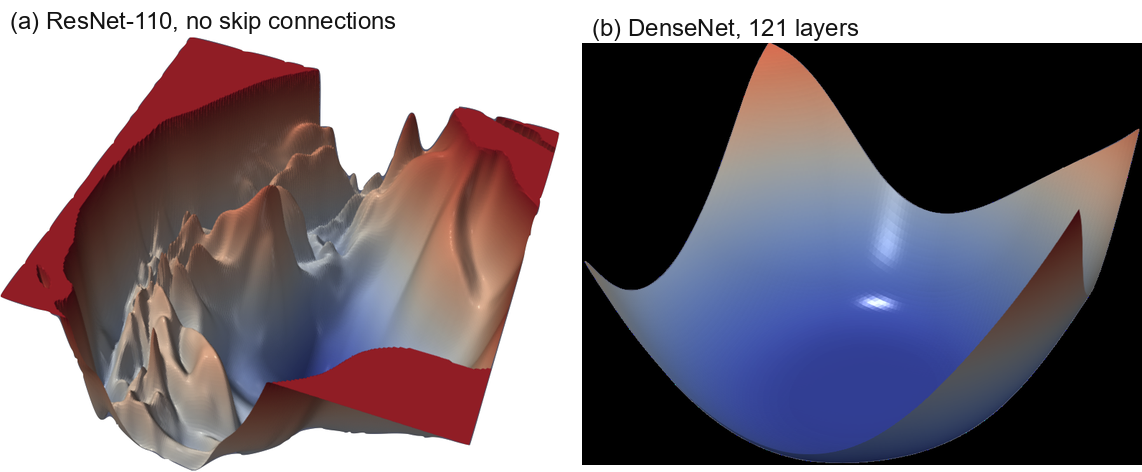
Shortcut Connections to the Rescue. Shortcut connections have a dramatic effect of the geometry of the loss functions. In Figure Figure 5, we see that residual connections prevent the transition to chaotic behavior as depth increases. In fact, the width and shape of the 0.1-level contour is almost identical for the 20- and 110-layer networks. Interestingly, the effect of skip connections seems to be most important for deep networks. For the more shallow networks (ResNet-20 and ResNet-20-noshort), the effect of skip connections is fairly unnoticeable. However residual connections prevent the explosion of non-convexity that occurs when networks get deep. This effect seems to apply to other kinds of skip connections as well; Figure Figure 4 show the loss landscape of DenseNet, which shows no noticeable non-convexity.

Shortcut Connections to the Rescue. Shortcut connections 对损失函数几何具有显著影响。 在 图5 中，我们看到 residual connections 会随着深度增加而阻止向混沌行为的转变。 事实上，20 层和 110 层网络的 0.1-level contour 的宽度和形状几乎相同。 有趣的是，skip connections 的影响似乎对深层网络最为重要。 对于较浅的网络（ResNet-20 和 ResNet-20-noshort），skip connections 的影响相当不明显。 然而，residual connections 阻止了网络变深时发生的非凸性爆炸。 这种效应似乎也适用于其他类型的 skip connections；图4 展示了 DenseNet 的损失景观，其中没有可见的非凸性。

图6：Wide-ResNet-56 on CIFAR-10 both with shortcut connections (top) and without (bottom). The label $k=2$ means twice as many filters per layer. Test error is reported below each figure.

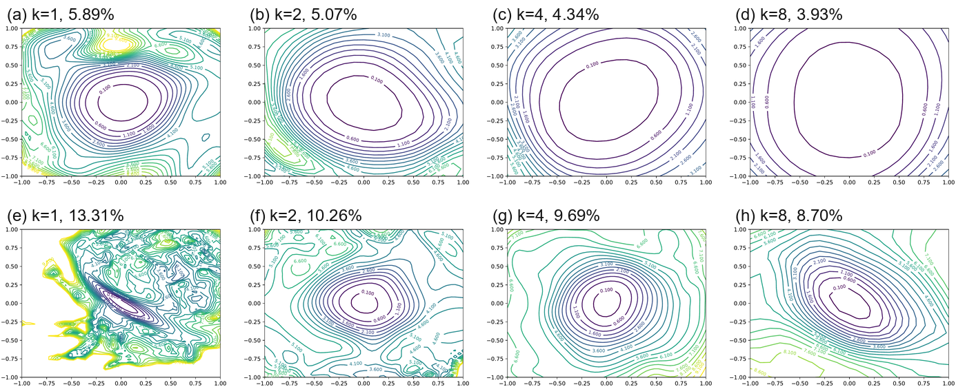
Wide Models vs Thin Models. To see the effect of the number of convolutional filters per layer, we compare the narrow CIFAR-optimized ResNets (ResNet-56) with Wide-ResNets by multiplying the number of filters per layer by $k=2,4,$ and $8$. From Figure Figure 6, we see that the wider models have loss landscapes with no noticeable chaotic behavior. Increased network width resulted in flat minima and wide regions of apparent convexity. We see that increased width prevents chaotic behavior, and skip connections dramatically widen minimizers. Finally, note that sharpness correlates extremely well with test error.

Wide Models vs Thin Models. 为考察每层卷积 filter 数量的影响，作者通过将每层 filter 数乘以 $k=2,4,$ 和 $8$，比较窄的 CIFAR 优化 ResNets（ResNet-56）与 Wide-ResNets。 从 图6 可以看到，更宽的模型具有没有明显混沌行为的损失景观。 增加网络宽度会产生平坦极小值和大片表观凸区域。 我们看到，增加宽度可以防止混沌行为，而 skip connections 会显著拓宽极小值点。 最后，请注意，尖锐程度与测试误差极其良好地相关。

Implications for Network Initialization. One interesting property seen in Figure Figure 5 is that loss landscapes for all the networks considered seem to be partitioned into a well-defined region of low loss value and convex contours, surrounded by a well-defined region of high loss value and non-convex contours. This partitioning of chaotic and convex regions may explain the importance of good initialization strategies, and also the easy training behavior of "good" architectures. When using normalized random initialization strategies such as those proposed by Glorot and Bengio, typical neural networks attain an initial loss value less than 2.5. The well behaved loss landscapes in Figure Figure 5 (ResNets, and shallow VGG-like nets) are dominated by large, flat, nearly convex attractors that rise to a loss value of 4 or greater. For such landscapes, a random initialization will likely lie in the "well- behaved" loss region, and the optimization algorithm might never "see" the pathological non-convexities that occur on the high-loss chaotic plateaus. Chaotic loss landscapes (ResNet-56/110-noshort) have shallower regions of convexity that rise to lower loss values. For sufficiently deep networks with shallow enough attractors, the initial iterate will likely lie in the chaotic region where the gradients are uninformative. In this case, the gradients "shatter", and training is impossible. SGD was unable to train a 156 layer network without skip connections (even with very low learning rates), which adds weight to this hypothesis.

对网络初始化的启示。 图5 中一个有趣性质是，所考虑所有网络的损失景观似乎都被划分为一个明确的低损失值和凸等高线区域，其外部被一个明确的高损失值和非凸等高线区域包围。 这种混沌区域和凸区域的划分，可能解释良好初始化策略的重要性，也解释“好”架构的易训练行为。 当使用 Glorot 和 Bengio 提出的 normalized random initialization 策略时，典型神经网络的初始损失值低于 2.5。 图5 中表现良好的损失景观（ResNets 和浅层 VGG-like 网络）由大型、平坦、近似凸的 attractors 主导，这些 attractors 会上升到 4 或更高的损失值。 对于这样的景观，随机初始化很可能落在“well-behaved”损失区域，优化算法可能永远“看不到”高损失混沌平台上发生的病态非凸性。 混沌损失景观（ResNet-56/110-noshort）具有更浅的凸区域，并上升到较低的损失值。 对于足够深且 attractors 足够浅的网络，初始迭代点很可能位于梯度不提供信息的混沌区域。 在这种情况下，梯度会“shatter”，训练不可能进行。 SGD 无法训练一个没有 skip connections 的 156 层网络（即使使用非常低的学习率），这为该假设增加了证据。

Landscape Geometry Affects Generalization. Both Figures Figure 5 and Figure 6 show that landscape geometry has a dramatic effect on generalization. First, note that visually flatter minimizers consistently correspond to lower test error, which further strengthens our assertion that filter normalization is a natural way to visualize loss function geometry. Second, we notice that chaotic landscapes (deep networks without skip connections) result in worse training and test error, while more convex landscapes have lower error values. In fact, the most convex landscapes (Wide-ResNets in the top row of Figure Figure 6), generalize the best of all, and show no noticeable chaotic behavior.

景观几何影响泛化。 图5 和 图6 都表明，景观几何对泛化具有显著影响。 首先，请注意，视觉上更平坦的极小值点始终对应更低的测试误差，这进一步强化了作者的论断：filter normalization 是可视化损失函数几何的一种自然方式。 其次，作者注意到，混沌景观（没有 skip connections 的深层网络）会导致更差的训练误差和测试误差，而更凸的景观具有更低的误差值。 事实上，最凸的景观（图6 顶行的 Wide-ResNets）泛化最好，并且没有明显混沌行为。

A note of caution: Are we really seeing convexity? We are viewing the loss surface under a dramatic dimensionality reduction, and we need to be careful how we interpret these plots. One way to measure the level of convexity in a loss function is to compute the principle curvatures, which are simply eigenvalues of the Hessian. A truly convex function has non-negative curvatures (a positive semi-definite Hessian), while a non-convex function has negative curvatures. It can be shown that the principle curvatures of a dimensionality reduced plot (with random Gaussian directions) are weighted averages of the principle curvatures of the full-dimensional surface (where the weights are Chi-square random variables).

提醒：我们真的看到凸性了吗？ 我们是在剧烈降维后观察损失曲面，因此需要谨慎解释这些图。 衡量损失函数凸性水平的一种方法是计算 principal curvatures，它们就是 Hessian 的特征值。 真正凸的函数具有非负曲率（正半定 Hessian），而非凸函数具有负曲率。 可以证明，降维图（使用随机高斯方向）的 principal curvatures 是全维曲面的 principal curvatures 的加权平均（其中权重为 Chi-square 随机变量）。

This has several consequences. First of all, if non-convexity is present in the dimensionality reduced plot, then non-convexity must be present in the full-dimensional surface as well. However, apparent convexity in the low-dimensional surface does not mean the high-dimensional function is truly convex. Rather it means that the positive curvatures are dominant (more formally, the mean curvature, or average eigenvalue, is positive).

这有若干后果。 首先，如果降维图中存在非凸性，那么全维曲面中也必然存在非凸性。 然而，低维曲面中的表观凸性并不意味着高维函数真正凸。 相反，它意味着正曲率占主导（更正式地说，mean curvature，或平均特征值，为正）。

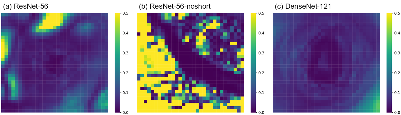
While this analysis is reassuring, one may still wonder if there is significant "hidden" non-convexity that these visualizations fail to capture. To answer this question, we calculate the minimum and maximum eigenvalues of the Hessian, ${\lambda }_{min}$ and ${\lambda }_{max}.$ We compute these using an implicitly restarted Lanczos method that requires only Hessian-vector products (which are calculated directly using automatic differentiation), and does not require an explicit representation of the Hessian or its factorization. Figure Figure 7 maps the ratio $|{\lambda }_{min}/{\lambda }_{max}|$ across the loss surfaces studied above (using the same minimizer and the same random directions). Blue color indicates a more convex region (near-zero negative eigenvalues relative to the positive eigenvalues), while yellow indicates significant levels of negative curvature. We see that the convex-looking regions in our surface plots do indeed correspond to regions with insignificant negative eigenvalues (i.e., there are not major non-convex features that the plot missed), while chaotic regions contain large negative curvatures. For convex-looking surfaces like DenseNet, the negative eigenvalues remain extremely small (less than 1% the size of the positive curvatures) over a large region of the plot.

虽然这一分析令人安心，但人们仍可能想知道，是否存在这些可视化未能捕捉到的显著“hidden”非凸性。 为回答这个问题，作者计算 Hessian 的最小和最大特征值 ${\lambda }_{min}$ 和 ${\lambda }_{max}$。 作者使用 implicitly restarted Lanczos 方法计算这些值，该方法只需要 Hessian-vector products（直接通过 automatic differentiation 计算），不需要 Hessian 的显式表示或分解。 图7 在上述研究的损失曲面上（使用相同极小值点和相同随机方向）映射比值 $|{\lambda }_{min}/{\lambda }_{max}|$。 蓝色表示更凸的区域（相对于正特征值，负特征值接近零），而黄色表示显著的负曲率水平。 可以看到，作者曲面图中看起来凸的区域确实对应于负特征值不显著的区域（即图没有漏掉主要非凸特征），而混沌区域包含大的负曲率。 对于 DenseNet 这类看起来凸的曲面，在图中的大区域内，负特征值仍然极小（小于正曲率大小的 1%）。

图7：For each point in the filter-normalized surface plots, we calculate the maximum and minimum eigenvalue of the Hessian, and map the ratio of these two.

7. Visualizing Optimization Paths

Finally, we explore methods for visualizing the trajectories of different optimizers. For this application, random directions are ineffective. We will provide a theoretical explanation for why random directions fail, and explore methods for effectively plotting trajectories on top of loss function contours.

最后，作者探索可视化不同优化器轨迹的方法。 对于这一应用，随机方向是无效的。 作者将提供随机方向失败原因的理论解释，并探索在损失函数等高线上有效绘制轨迹的方法。

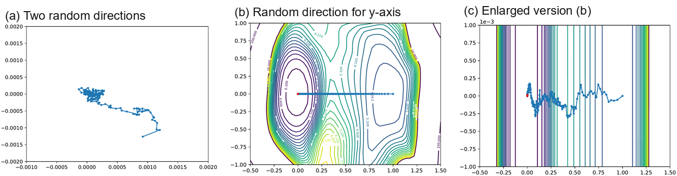
Several authors have observed that random directions fail to capture the variation in optimization trajectories. Example failed visualizations are depicted in Figure Figure 8. In Figure Figure 8(a), we see the iterates of SGD projected onto the plane defined by two random directions. Almost none of the motion is captured (notice the super-zoomed-in axes and the seemingly random walk). This problem was noticed by Goodfellow et al., who then visualized trajectories using one direction that points from initialization to solution, and one random direction. This approach is shown in Figure Figure 8(b). As seen in Figure Figure 8(c), the random axis captures almost no variation, leading to the (misleading) appearance of a straight line path.

已有若干作者观察到，随机方向无法捕捉优化轨迹中的变化。 失败可视化示例如 图8 所示。 在 图8(a) 中，我们看到 SGD 的迭代点被投影到由两个随机方向定义的平面上。 几乎没有任何运动被捕捉到（注意极度放大的坐标轴和看似随机游走的路径）。 Goodfellow 等人注意到了这个问题，随后使用一个从初始化指向解的方向和一个随机方向来可视化轨迹。 这种方法如 图8(b) 所示。 如 图8(c) 所示，随机轴几乎没有捕捉到任何变化，从而导致路径看起来像一条直线的（误导性）外观。

图8：Ineffective visualizations of optimizer trajectories. These visualizations suffer from the orthogonality of random directions in high dimensions.

7.1 Why Random Directions Fail: Low-Dimensional Optimization Trajectories

It is well-known that two random vectors in a high dimensional space will be nearly orthogonal with high probability. In fact, the expected cosine similarity between Gaussian random vectors in $n$ dimensions is roughly $\sqrt{2/(\pi n)}$ (Goldstein and Studer, Lemma 5).

众所周知，高维空间中的两个随机向量会以高概率近乎正交。 事实上，$n$ 维中高斯随机向量之间的期望 cosine similarity 约为 $\sqrt{2/(\pi n)}$（Goldstein 和 Studer，引理 5）。

This is problematic when optimization trajectories lie in extremely low dimensional spaces. In this case, a randomly chosen vector will lie orthogonal to the low-rank space containing the optimization path, and a projection onto a random direction will capture almost no variation. Figure Figure 8(b) suggests that optimization trajectories are low-dimensional because the random direction captures orders of magnitude less variation than the vector that points along the optimization path. Below, we use PCA directions to directly validate this low dimensionality, and also to produce effective visualizations.

当优化轨迹位于极低维空间中时，这会带来问题。 在这种情况下，随机选择的向量会与包含优化路径的低秩空间正交，而投影到随机方向几乎无法捕捉任何变化。 图8(b) 表明优化轨迹是低维的，因为随机方向捕捉到的变化量比沿优化路径方向的向量小几个数量级。 下面，作者使用 PCA directions 直接验证这种低维性，同时生成有效的可视化。

7.2 Effective Trajectory Plotting using PCA Directions

To capture variation in trajectories, we need to use non-random (and carefully chosen) directions. Here, we suggest an approach based on PCA that allows us to measure how much variation we've captured; we also provide plots of these trajectories along the contours of the loss surface.

为了捕捉轨迹中的变化，我们需要使用非随机（且精心选择的）方向。 这里，作者提出一种基于 PCA 的方法，使我们能够衡量捕捉了多少变化；作者还提供了这些轨迹沿损失曲面等高线的图。

Let ${\theta }_i$ denote model parameters at epoch $i,$ and the final parameters after $n$ epochs of training are denoted ${\theta }_n$. Given $n$ training epochs, we can apply PCA to the matrix

$$M=[{\theta }_0-{\theta }_n;\cdots ;{\theta }_{n-1}-{\theta }_n],$$

and then select the two most explanatory directions. Optimizer trajectories (blue dots) and loss surfaces along PCA directions are shown in Figure Figure 9. Epochs where the learning rate was decreased are shown as red dots. On each axis, we measure the amount of variation in the descent path captured by that PCA direction.

令 ${\theta }_i$ 表示第 $i$ 个 epoch 的模型参数，训练 $n$ 个 epochs 后的最终参数表示为 ${\theta }_n$。 给定 $n$ 个训练 epochs，我们可以对如下矩阵应用 PCA：

$$M=[{\theta }_0-{\theta }_n;\cdots ;{\theta }_{n-1}-{\theta }_n],$$

然后选择解释性最强的两个方向。 优化器轨迹（蓝点）以及沿 PCA 方向的损失曲面如 图9 所示。 学习率降低的 epochs 显示为红点。 在每条轴上，作者测量该 PCA 方向捕捉到的下降路径变化量。

图9：Projected learning trajectories use normalized PCA directions for VGG-9. The left plot in each subfigure uses batch size 128, and the right one uses batch size 8192.

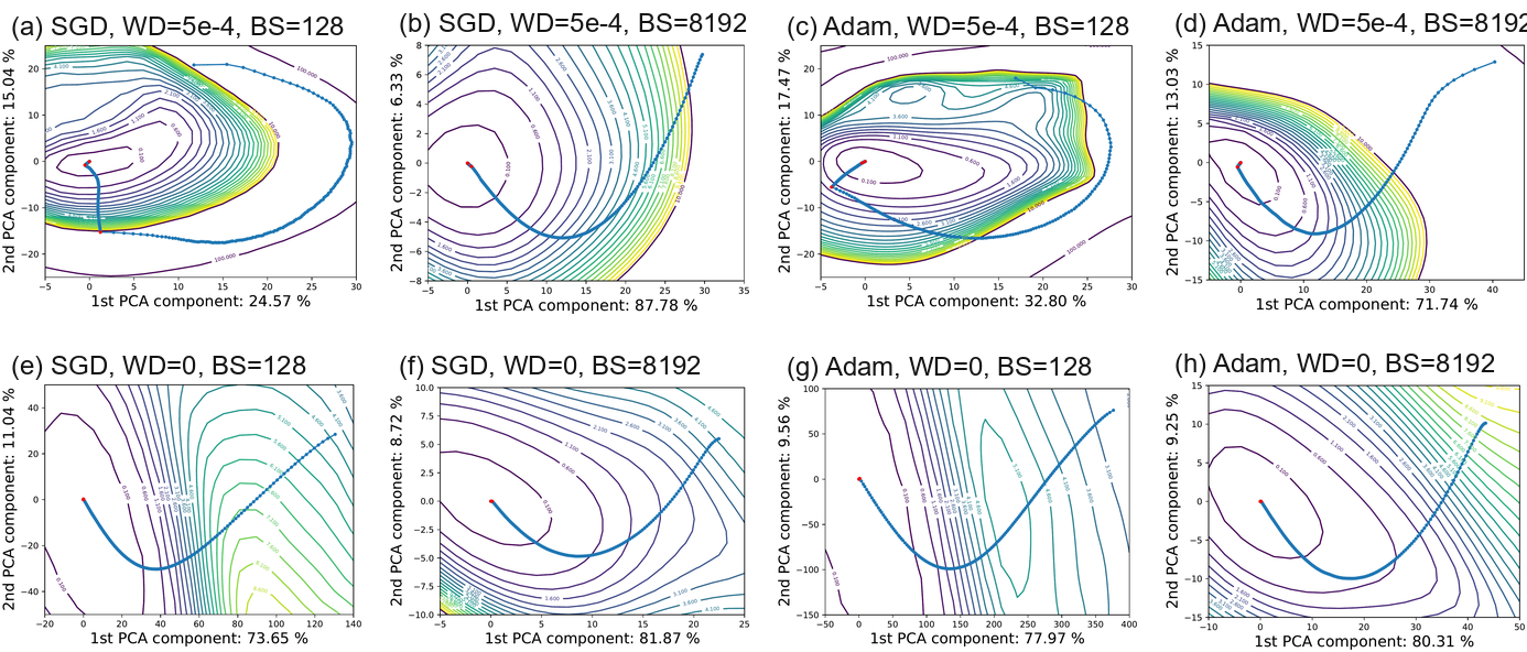
At early stages of training, the paths tend to move perpendicular to the contours of the loss surface, i.e., along the gradient directions as one would expect from non-stochastic gradient descent. The stochasticity becomes fairly pronounced in several plots during the later stages of training. This is particularly true of the plots that use weight decay and small batches (which leads to more gradient noise, and a more radical departure from deterministic gradient directions). When weight decay and small batches are used, we see the path turn nearly parallel to the contours and "orbit" the solution when the stepsize is large. When the stepsize is dropped (at the red dot), the effective noise in the system decreases, and we see a kink in the path as the trajectory falls into the nearest local minimizer.

在训练早期阶段，路径倾向于垂直于损失曲面的等高线移动，即沿着梯度方向移动，这正是非随机梯度下降所预期的行为。 在训练后期阶段，若干图中的随机性变得相当明显。 这在使用 weight decay 和 small batches 的图中尤其如此（这会导致更多梯度噪声，并更大幅度偏离确定性梯度方向）。 当使用 weight decay 和 small batches 时，可以看到在 stepsize 较大时，路径转为几乎平行于等高线，并围绕解“orbit”。 当 stepsize 下降时（红点处），系统中的有效噪声减少，可以看到轨迹落入最近局部极小值点时路径出现一个拐点。

Finally, we can directly observe that the descent path is very low dimensional: between 40% and 90% of the variation in the descent paths lies in a space of only 2 dimensions. The optimization trajectories in Figure Figure 9 appear to be dominated by movement in the direction of a nearby attractor. This low dimensionality is compatible with the observations in Section 6, where we observed that non-chaotic landscapes are dominated by wide, nearly convex minimizers.

最后，我们可以直接观察到下降路径非常低维：下降路径中 40% 到 90% 的变化位于仅有 2 维的空间中。 图9 中的优化轨迹似乎由朝向附近 attractor 的方向上的运动主导。 这种低维性与第 6 节中的观察相容，在那里作者观察到非混沌景观由宽而近似凸的极小值点主导。

8. Conclusion

We presented a visualization technique that provides insights into the consequences of a variety of choices facing the neural network practitioner, including network architecture, optimizer selection, and batch size. Neural networks have advanced dramatically in recent years, largely on the back of anecdotal knowledge and theoretical results with complex assumptions. For progress to continue to be made, a more general understanding of the structure of neural networks is needed. Our hope is that effective visualization, when coupled with continued advances in theory, can result in faster training, simpler models, and better generalization.

作者提出了一种可视化技术，它能够洞察神经网络实践者面临的多种选择所带来的后果，包括网络架构、优化器选择和 batch size。 近年来，神经网络取得了巨大进步，这在很大程度上依赖经验性知识和带有复杂假设的理论结果。 要继续取得进展，就需要对神经网络结构有更一般的理解。 作者希望，有效可视化与理论的持续进展相结合，能够带来更快训练、更简单模型和更好泛化。